



Author: Vesselin Tzvetkov, Principal Security Engineer and Security Advisor
Co- Author: Andre Mohr, Cloud Security Consultant
The Google Security Operations (SecOps) platform provides a wide set of powerful AI features to improve the effectiveness of incident detection and response, such as natural language search query and detection rule creation, case investigation summaries, and a multi-turn chat assistant for investigations. However, in certain SOC environments, operating within specialized industries can encounter advanced threat vectors that benefit from customized analytical modeling and AI models. This article shows how to use the Google SecOps BigQuery Export feature to extend out-of-the-box capabilities and detect more targeted attacks.
This post details the first of two machine learning (ML) pilots created, focusing on using BigQuery ML to build custom time-series forecasting models directly from Universal Data Model (UDM) events to analyze device telemetry. As initially developing these custom pipelines as well as training models and maintaining the model is resource and cost intensive,we recommend using these only when off-the-shelf Google SecOps cannot cover specialized use cases, such as Operational Technology (OT) or industrial environments, especially when those systems represent critical "crown jewel" assets or carry high security requirements.
Use Case
Let us define our concrete representative use case that we will implement:
Goal: Detect statistical anomalies in device activities count (log types NETWORK_TELEMETRY_A or NETWORK_TELEMETRY_B). An alert will be triggered when the current message count deviates significantly from the estimated projection build from past device activities. The projection (apriori estimation) is a device profile that considers data trends (the long-term direction of the data) as well as seasonality and cycle behaviors over a rolling historical lookback window. The profile is built in an unsupervised machine learning (ML) without manual labeling or tuning needed.
For example: an IoT/OT device is expected to send 5–7K messages with 99% certainly (0.99 confidence interval) between 4 PM and 5 PM based based on its historical baseline; we want to detect deviations with a peak or dip magnitude factor of 5 standard division and a 99,99% certainty. If we receive just a few messages (critical dip) or 1 million (an extreme spike), we want to detect this. Additionally, we want to build this baseline profile per individual device using unsupervised ML (no human data labeling), rather than grouping devices together.
Implementation
The following 4 steps were used to build a holistic architecture, to implement custom machine learning alerts and feed them back to Google SecOps.
-
Telemetry Export: Continuously streaming structured enterprise log data from the core security platform into dedicated analytics tables.
-
Baselining: Training independent, custom prediction models for every individual device identity simultaneously.
-
Deviation Detection: Evaluating live operational feeds against the trained custom models to identify significant shifts.
-
Alert Ingestion: Using Cloud Run Functions to trigger periodic evaluation of events against models to identify outliers and to route them to Google SecOps to trigger downstream SOAR playbooks.
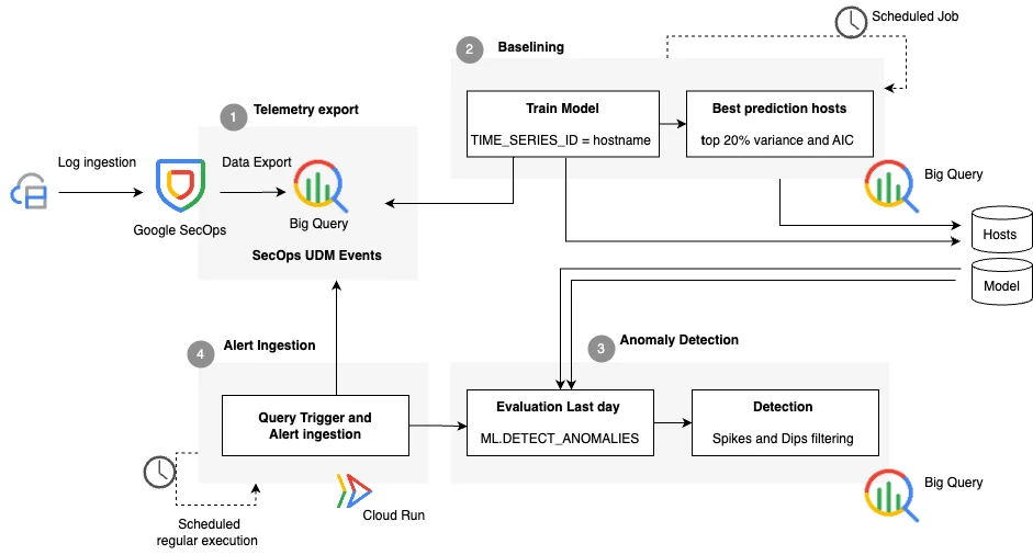
Figure 1: Information Flow Architecture
1. Telemetry Export
Google SecOps provides a built-in streaming mechanism to continuously export Universal Data Model (UDM) events into a Google SecOps BigQuery via Google SecOps BigQuery Export, which can be used later on to run custom model training and alerting.
The Google SecOps BigQuery Export can be done in multiple ways depending on your setup, need and license type.
-
Export to a self-managed BigQuery project that you own and manage for Google SecOps Enterprise customers. You can link your own Google Cloud project to your Google SecOps instance and independently manage IAM permissions with no dependency on Google-managed settings. You can also enable and configure in Google SecOps, see Figure 2.
-
Export to a Google-managed BigQuery project to route telemetry directly into managed BigQuery for Google SecOps Enterprise Plus customers.
-
Advanced BigQuery export to access your security data in near-real-time through a fully managed, streaming data pipeline for Google SecOps Enterprise Plus customers.
Even when utilizing the Google-managed database via Enterprise Plus, a customer-owned Google Cloud Project and dedicated BigQuery database remain a requirement for machine learning execution. Because the provided linked dataset is strictly read-only, custom model creation statements cannot write data or store output artifacts back inside the managed tenant project. A dedicated BigQuery instance must be used as the execution environment, querying the read-only source telemetry fields while saving the generated machine learning models, weights, and scoring tables to own self-managed datasets.
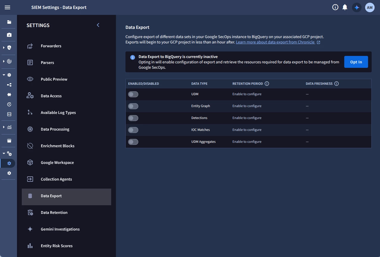
Figure 2: Screenshot of Google SecOps Data Export configuration
2. Baselining
The initial technical implementation focuses on transforming continuous streams of Universal Data Model (UDM) events into an aggregated time-series matrix that a machine learning model can ingest. The raw inputs consist of system logs containing source identifiers, system event records, and epoch timestamps. The structured output targets a unified analytics view that tracks the exact volume of transactions compiled per device hostname, per period (e.g. in the pilot case per hour).
To establish individual baselines across a large group of sources without building separate training pipelines, the solution utilizes BigQuery ML's capability, specifically the ARIMA_PLUS model. ARIMA_PLUS is natively built into the Google Cloud BigQuery ML (BQML) engine, allowing users to train complex time-series models and detect anomalies in an unsupervised way using simple, standard SQL queries. The model considers trends (the long-term direction of the data) and seasonality (such as hourly, daily, weekly, or yearly cycles), holiday effects and its scalability makes it excellent for anomaly detection in an inexpensive way.
The following statement can be executed within the BigQuery environment to orchestrate parallel model training across all log sources:
CREATE OR REPLACE MODEL `enterprise_security_ml.device_telemetry_anomaly_model`
OPTIONS (
  MODEL_TYPE = 'ARIMA_PLUS',
  TIME_SERIES_TIMESTAMP_COL = 'activity_hour',
  TIME_SERIES_DATA_COL = 'activity_count',
  TIME_SERIES_ID_COL = 'host_id',
  DATA_FREQUENCY = 'HOURLY'
) AS (
  WITH AggregatedData AS (
    SELECT
      principal.hostname AS host_id,
      TIMESTAMP_TRUNC(TIMESTAMP_SECONDS(metadata.event_timestamp.seconds), HOUR) AS activity_hour,
      COUNT(*) AS activity_count
    FROM
      `enterprise_secops_dataset.datalake.events`
    WHERE
      principal.hostname IS NOT NULL
      AND (metadata.log_type = 'NETWORK_TELEMETRY_A' OR metadata.log_type = 'NETWORK_TELEMETRY_B')
    GROUP BY
      host_id,
      activity_hour
  ),
  TrainingWindow AS (
    SELECT
      TIMESTAMP_SUB(TIMESTAMP_TRUNC(CURRENT_TIMESTAMP(), DAY), INTERVAL 2 DAY) AS training_end_exclusive,
      TIMESTAMP_SUB(TIMESTAMP_TRUNC(CURRENT_TIMESTAMP(), DAY), INTERVAL 16 DAY) AS training_start_inclusive
  )
  SELECT
    t1.host_id,
    t1.activity_hour,
    t1.activity_count
  FROM
    AggregatedData AS t1
  CROSS JOIN
    TrainingWindow AS t2
  WHERE
    t1.activity_hour >= t2.training_start_inclusive
    AND t1.activity_hour < t2.training_end_exclusive
);
The core structural configurations used in this technical implementation include:
-
MODEL_TYPE: Specifying ARIMA_PLUS invokes a time-series modeling pipeline that performs pre-training steps including handling duplicate timestamps, interpolating missing values, detecting historical anomalies, and selecting ARIMA parameters via auto-tuning.
-
TIME_SERIES_ID_COL: By mapping the time series to host_id, BigQuery ML is instructed to dynamically partition the dataset and fit a completely independent, localized ARIMA model for each unique identifier. Instead of writing custom orchestration code to loop through thousands of devices or maintaining separate ML pipelines for every endpoint, this single configuration handles the concurrent training of distinct baseline models across all device sources within one SQL execution.
-
TrainingWindow: This expression isolates a shifting 14-day data window for historical training, intentionally imposing a 2-day buffer gap relative to the execution runtime. The first buffered day is used for the "best host" evaluation, while the final day of the buffer is reserved for the first active prediction pass against current telemetry. You can adjust the time windows depending on your exact use case and use these values as samples.
Filtering for Usable Models (The "Best Prediction Hosts" approach)
Not all hardware devices generate continuous or predictable log volumes. Following the training execution, the quality of the generated models must be evaluated (utilizing the ML.EVALUATE function) to assess variance and error metrics for each specific source using the reserved buffer data. Devices, which fail to meet minimum predictability thresholds, are filtered out, generating an optimized best_prediction_hosts baseline table. This filtering step ensures that downstream anomaly detection is performed on more stable sources to reduce false positive alerts.
3. Anomaly Detection
Once the device-specific baselines are established, the pipeline transitions to active prediction and validation. The scoring query can be used to continuously evaluate live events against the computed forecasting thresholds using the ML.DETECT_ANOMALIES function. With this approach, the system can be used to isolate high-priority security events, such as sudden log silence ("Deep Dips") or extended telemetry occurrence due to configuration modifications ("High Peaks").
The following detection query can be utilized to evaluate system telemetry over the trailing 48-hour window, specifically joining against the pre-filtered best_prediction_hosts table:
DECLARE peak_magnitude_factor FLOAT64 DEFAULT 5.0;
DECLARE dip_significance_threshold FLOAT64 DEFAULT 5.0;

WITH AnomalyResults AS (
  SELECT * FROM ML.DETECT_ANOMALIES(
    MODEL `enterprise_security_ml.device_telemetry_anomaly_model`,
    STRUCT(0.999 AS anomaly_prob_threshold),
    (
      SELECT principal.hostname AS host_id,
             TIMESTAMP_TRUNC(TIMESTAMP_SECONDS(metadata.event_timestamp.seconds), HOUR) AS activity_hour,
             COUNT(*) AS activity_count
      FROM `enterprise_secops_dataset.datalake.events`
      WHERE principal.hostname IS NOT NULL AND (metadata.log_type = 'NETWORK_TELEMETRY_A' OR metadata.log_type = 'NETWORK_TELEMETRY_B')
      GROUP BY host_id, activity_hour
    )
  )
  WHERE activity_hour >= TIMESTAMP_SUB(TIMESTAMP_TRUNC(CURRENT_TIMESTAMP(), DAY), INTERVAL 2 DAY)
),
BestHosts AS (SELECT host_id FROM `enterprise_security_ml.best_prediction_hosts`)

SELECT ar.host_id, ar.activity_hour, ar.activity_count, ar.upper_bound, ar.lower_bound, ar.anomaly_probability,
       CASE
         WHEN ar.is_anomaly = TRUE AND ((ar.upper_bound > 0 AND ar.activity_count > (ar.upper_bound * peak_magnitude_factor)) OR (ar.upper_bound <= 0 AND ar.activity_count > 0)) THEN 'High Peak'
         WHEN ar.activity_count = 0 AND ar.upper_bound > dip_significance_threshold THEN 'Deep Dip'
       END AS anomaly_type
FROM AnomalyResults AS ar
JOIN BestHosts AS bh ON ar.host_id = bh.host_id
WHERE (ar.is_anomaly = TRUE AND ((ar.upper_bound > 0 AND ar.activity_count > (ar.upper_bound * peak_magnitude_factor)) OR (ar.upper_bound <= 0 AND ar.activity_count > 0)))
   OR (ar.activity_count = 0 AND ar.upper_bound > dip_significance_threshold)
ORDER BY anomaly_type, ar.anomaly_probability DESC;
Tuning & Adaptation
Deploying time-series forecasting across live corporate environments initially creates false positives e.g. due to unexpected routine maintenance. The presented solution supports fine-tuning of configurations to establish appropriate alert thresholds. In this pilot, the peak_magnitude_factor can be adjusted to ignore benign traffic bursts, and the dip_significance_threshold can be elevated to isolate critical infrastructure drop-offs where communication drops significantly.
4. Alert Ingestion
In order to continuously, periodically run validations against new telemetry data, Cloud Run Functions triggered by Cloud Scheduler can be used to execute the BigQuery workflow and ingest events into Google SecOps SIEM.
The following Python code shows a simplified code snippet:
# [...] (Imports, environment variables and helper functions)

@app.route('/trigger-scoring', methods=['POST'])
def trigger_scoring():
    # [...] (Initial setup and validation)

    try:
        # [...] Authenticate using Application Default Credentials (ADC)

        # Execute the Anomaly Detection Query
        BQ_ANOMALY_QUERY = os.environ.get("BQ_ANOMALY_QUERY")
        query_job = bq_client.query(BQ_ANOMALY_QUERY)
        results = query_job.result()

        # Batch and Ingest Anomalies to SecOps
        chronicle_url = "https://malachiteingestion-pa.googleapis.com/v2/unstructuredlogentries:batchCreate"
        log_batch = []

        for row in results:
            # Map the BigQuery row directly to the SecOps alert schema
            alert_payload = {
                "host_id": row.host_id,
                "anomaly_type": row.anomaly_type,
                "activity_hour": str(row.activity_hour),
                "actual_count": row.activity_count,
                "expected_upper_bound": row.upper_bound,
                "expected_lower_bound": row.lower_bound,
                "anomaly_probability": row.anomaly_probability,
                "source_model": "bqml_device_telemetry_anomaly_model"
            }

            log_entry = {
                "log_text": json.dumps(alert_payload),
                "parser_type": PARSER_TYPE
            }
            log_batch.append(log_entry)

            # Flush batch when size limit reached
            if len(log_batch) >= BATCH_SIZE:
                send_batch_to_chronicle(chronicle_url, CHRONICLE_CUSTOMER_ID, log_batch, authed_session)
                log_batch = []

        # [...]
Wrap-up
Building custom machine learning pipelines requires dedicated engineering effort, making it an appropriate solution when standard security products are not available for specialized systems or architectures, such as Operational Technology (OT) environments.
The advantage of this approach lies in the integration between Google SecOps and Google Cloud BigQuery. By leveraging BigQuery ML, security teams can execute parallel model training for thousands of individual device sources simultaneously. This capability allows analysts to scale custom baseline creation efficiently and eliminates the need to build or manage complex data engineering pipelines.
Following some fine-tuning cycles to establish anomaly thresholds and filter for the best prediction hosts, the pilot provided valuable alerts. The predictive forecasting models successfully surfaced telemetry deviations and proved useful for identifying specific attacks but also critical gaps within the company’s internal change management processes.
The presented solution should just be seen as a pilot. There are multiple potential areas of improvement, including but not limited to:
-
Model Optimization: Refine baseline accuracy by evaluating alternative algorithms or tuning hyperparameters within the BigQuery ML creation statement.
-
Cost Efficiency: Running continuous analytics across a wide set of log data and device sources allows for further cost optimization considering the training frequency and included devices.
-
Expanded Use Cases: Establishing the shown architecture unlocks the ability to pilot other machine learning techniques as well (e.g. classification models). This might help to address a much broader range of complex predictive security challenges beyond just volume forecasting.
