
Over the past months, I've been experimenting with an innovation in Google SQL called pipe syntax (white paper). As the name implies, pipe syntax extends the Structured Query Language (SQL) by adding a piped data flow construct that will be immediately familiar to anyone who has experience with pipe-based or "flow" query languages like Search Processing Language (SPL) or Kusto Query Language (KQL). Recently, support for pipe syntax became generally available in Google Cloud BigQuery and Cloud Logging. It's time to share a first look at using Google SQL pipe syntax for analyzing security data.
Our Data
For the examples in this blog, we will use realistic (but anonymized/synthetic) security data exported from Google Security Operations (SecOps) to BigQuery. Google SecOps has parsed the data using the Unified Data Model schema (UDM). UDM parsing maps unstructured or semi-structured raw security events to a standard semantic taxonomy. It adds the structure necessary to store it efficiently in the rows and columns of relational database tables like those in BigQuery. While UDM data exported from Google SecOps provides convenient sample data for our examples, the techniques we cover are broadly applicable to any security data normalized to any schema.
Our examples use BigQuery, where we query the events table within the datalake dataset. These tables and datasets are created automatically during the export from Google SecOps. If you have questions about the semantic meanings of any column names (e.g., principal.ip), please refer to the UDM Field List.
Pipe Syntax 101
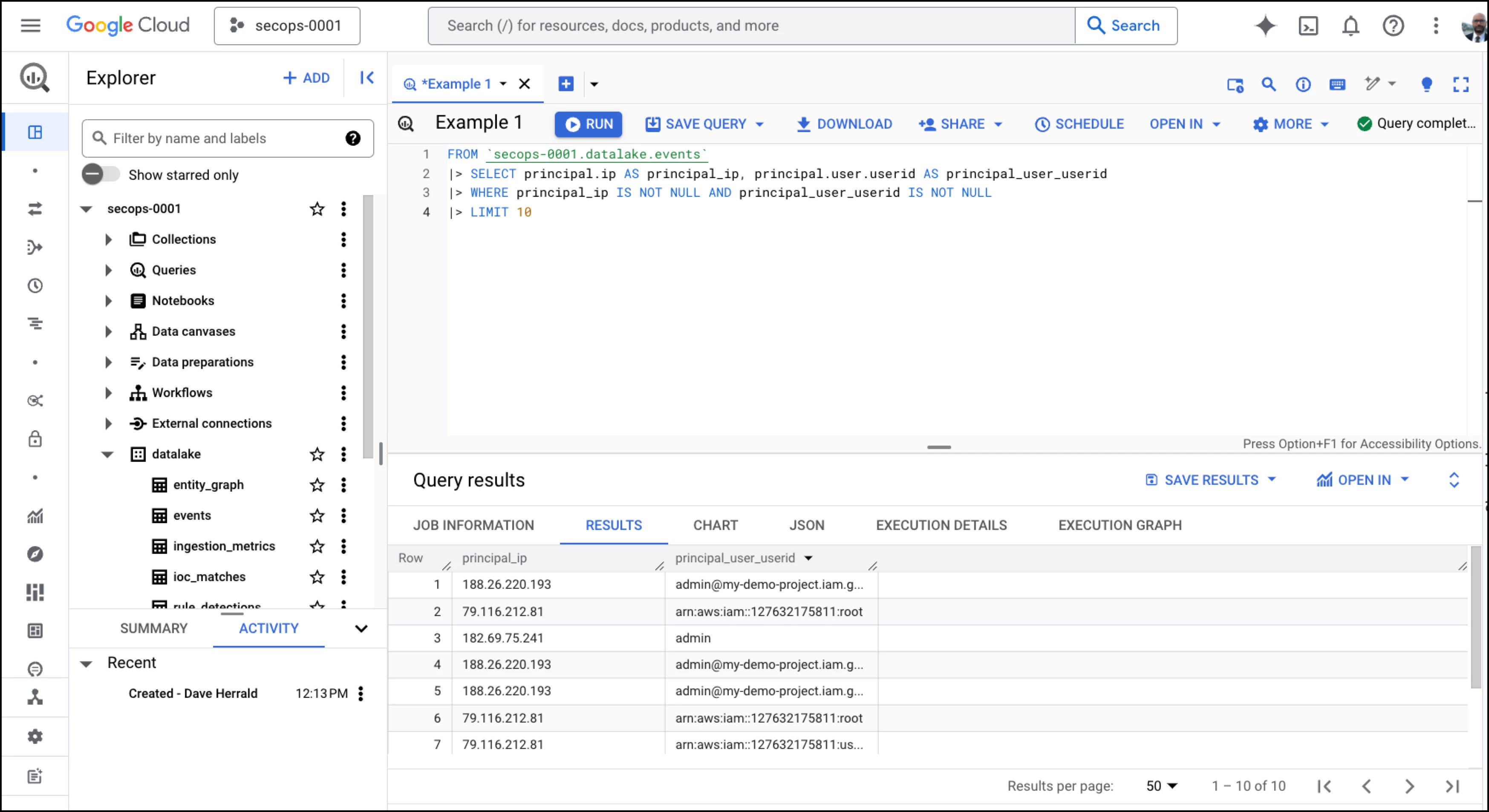
Let's jump in and look at pipe syntax in action. The first example shows a screenshot of the BigQuery interface in the Google Cloud Console. In the Explorer on the left, you can see the Google Cloud project name "secops-0001," the datalake dataset, and the events table, which we mentioned earlier. The pipe syntax query is highlighted in color, and the query results are shown at the bottom. In the following sections, we'll explain what this query is doing and present more practical examples. In this example, we show the interface you will most likely use when getting started.
Simple Pipe Syntax Example
One of the most significant benefits of using pipe syntax is readability. Queries are easy to follow, explain, and troubleshoot. To do so, proceed line-by-line from top to bottom. Let's do that for this query.
| Pipe Syntax Query, line-by-line | Explanation | |
| 1 | FROM `secops-0001.datalake.events` | Bootstrap this pipe syntax query with the full contents of our BigQuery events table. A standalone FROM clause is a good sign this is a pipe syntax query. It’s a massive table with millions or billions of rows and thousands of columns, but that’s ok. Security data schemas are almost always large and complex, but we’ll filter most of that out as we build up the query. |
| 2 | |> SELECT principal.ip AS ip, | Our first pipe operator is |> SELECT. indicated by the pipe character |> The |> SELECT operator reduces the number of columns we are working with from several thousand down to just two, and it gives each of them a friendly name. Both principal.ip and principal.user.userid are field names from the UDM event data model. The dots in these field names indicate the hierarchy UDM defines under its "principal" noun. |
| 3 | |> WHERE ip IS NOT NULL AND userid IS NOT NULL | Next, we use the |> WHERE pipe operator to filter out rows that don’t include the data we are looking for. Note that with pipe syntax, we can add more |> WHERE clauses after this one whenever the need arises. |
| 4 | |> LIMIT 10 | Finally, we use the >| LIMIT pipe operator to keep only the first ten output rows and discard the rest. |
Pipe syntax makes queries easy to understand and troubleshoot when broken down this way. Let's take a closer look at some details.
The Pipe Character and Operators
Google SQL defines the pipe character as |>. When you see |> in a Google SQL query, that's pipe syntax! The pipe character is followed by one or more keywords called pipe operators. Pipe operators are usually followed by arguments that vary depending on the operator. Our first example uses three pipe operators: |> SELECT, |> WHERE, and |> LIMIT.
Table In, Table Out
A key principle in Google SQL pipe syntax is that pipe operators take a table as input and produce a table as output. You can think of the data in your query flowing from top to bottom as a table whose shape and contents are transformed at each step. The pipe operators you choose and the order in which you apply them dictate precisely how this transformation works. You might alter the shape of the table by computing and adding new columns, dropping unnecessary columns, enriching the table's rows with data from other tables, sorting the rows, filtering the rows, or even aggregating rows into a summary table. This concept is the essence of Google SQL pipe syntax and most pipe-delimited or flow-based languages.
How is the first input table created to bootstrap the process? The pipe syntax authors allow for a standalone "FROM" clause, as shown in line 1 of the first example. Here, we provide the entire events table as the input to the first pipe operator.
Order Matters
In pipe syntax, the order of the pipe operators matters. It has a semantic meaning for the query. In practical terms, this order helps define precisely how the tabular data is transformed as it moves from one pipe operator to the next. The syntax also allows repeating the same pipe operator later in the same query. That capability will be familiar to users of other pipe-based languages but may not be so apparent to SQL experts or YARA-L users.
It's important to note that while pipe syntax allows you to express the query in a linear order, it still results in a declarative query. The query engine will still optimize and reorder the query, just as in standard SQL, to find the most efficient way to produce a semantically equivalent answer.
Results
At the end of the query, we are left with some tabular results. These can be used in typical security data analysis use cases like detection, alerting, investigation, or visualization/reporting. They can also become the basis of threat hunting hypotheses or be saved to a new table for later uses like enrichment or training for machine learning or AI applications.
Pipe Syntax is Still SQL!
When you start working with pipe syntax, it can be easy to forget that you are still writing SQL. Although it can feel like a completely different language, it's not. It's valid Google SQL. This point is emphasized by the pipe syntax authors in the conclusion of the SQL Pipe Paper (PDF linked above): "The resulting language is still SQL, but it's a better SQL. It's more flexible, more extensible, and easier to use."
Pipe syntax queries get processed by the same engine. They get optimized and maintain declarative semantics. Pipe syntax allows you to use the same language and tools for your data warehouse and other databases, even allowing you to do joins across disparate datasets. Pipe syntax enables you to take advantage of powerful features in SQL, such as views and user-defined functions (UDF), and even more powerful capabilities, such as table-valued functions (TVF). It leverages the impressive list of existing functions available in Google SQL, which allow for mathematical/arithmetic calculations, string manipulation, regular expressions, JSON handling, statistical analysis, date/time manipulation, and geographical calculations, to mention just a few.
It's also important to note that Google SQL pipe syntax is entirely additive to SQL. SQL experts need never write a single pipe character or even concern themselves with learning pipe syntax at all. Powerful constructs in SQL like "WITH" clauses, common table expressions (CTE), and subqueries still work as they always have. Pipe syntax represents a powerful new option, but it is just an option. No existing Google SQL features have been removed or deprecated.
Example - Top Talkers
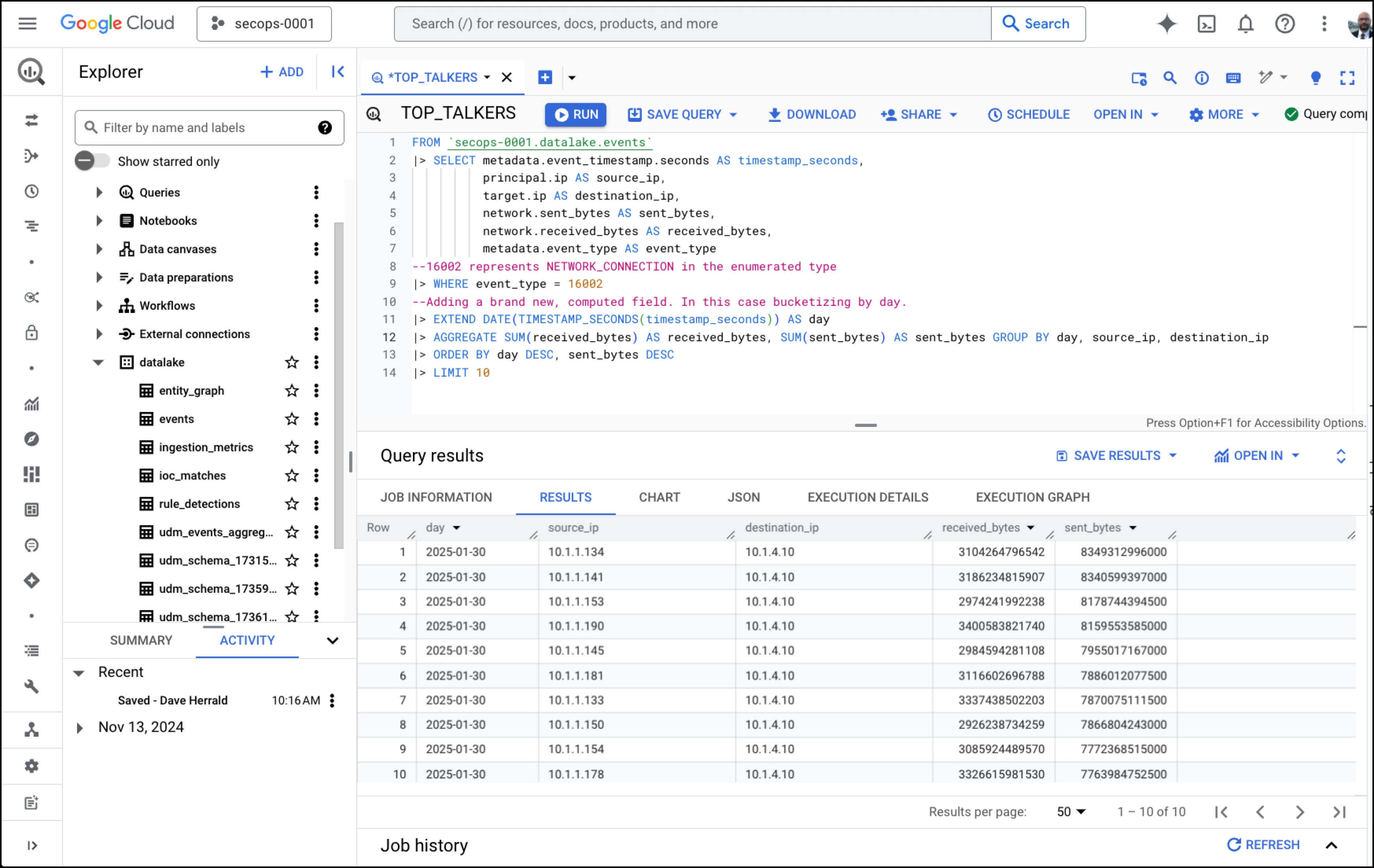
Here is a more useful example, one that takes advantage of several more features of pipe syntax. The query creates a list of network "Top Talkers." To do this, it computes the amount of data sent across a network between IP address pairs each day and sorts the results. Ultimately, the query returns the top ten most talkative pairs.
Example - Top Talkers
Let’s analyze the Top Talkers example line-by-line.
| Pipe Syntax Query, line-by-line | Explanation | |
| 1 | FROM `secops-0001.datalake.events` | Start the query with the entire events table. |
| 2 | |> SELECT | The |> SELECT pipe operator narrows the input table down to a smaller set of columns and assigns them shorter and more convenient names using “AS.” Note that pipe operators and their arguments can span multiple lines. |
| 3 | principal.ip AS source_ip, | |
| 4 | target.ip AS destination_ip, | |
| 5 | network.sent_bytes AS sent_bytes, | |
| 6 | network.received_bytes AS received_bytes, | |
| 7 | metadata.event_type AS event_type | |
| 8 | --16002 represents NETWORK_CONNECTION | Two dashes are a way to indicate comments in Google SQL queries. Comments are not specific to pipe |
| 9 | |> WHERE event_type = 16002 | 16002 is the integer associated with network connections in the UDM schema enumeration for metadata.event_type. |
| 10 | --Adding computed column. | More comments! |
| 11 | |> EXTEND | The |> EXTEND pipe operator adds a column to the table and names it “day.” In this case, |> EXTEND uses the “DATE” SQL function to convert a timestamp to a year-month-date format (yyyy-mm-dd.) |
| 12 | |> AGGREGATE | The ability to summarize or aggregate data is perhaps the most used capability in any query language. The |> AGGREGATE operator is used to compute aggregates in pipe syntax. In this case, we are summing the received and sent bytes columns and aggregating them by source_ip, destination_ip, and day. Aggregating converts individual rows into a summary where each row represents statistics for each day, source_ip, and destination_ip combination. |
| 13 | |> ORDER BY day DESC, sent_bytes DESC | Finally, we sort the aggregated rows in descending order by date and sub-sort by sent_bytes. |
| 14 | |> LIMIT 10 | The |> LIMIT pipe operator trims the sorted list to include just the first ten values, and voila! We have a helpful query for identifying top talkers on our network. |
Example - Multiple Failed Logins Followed by a Successful Login
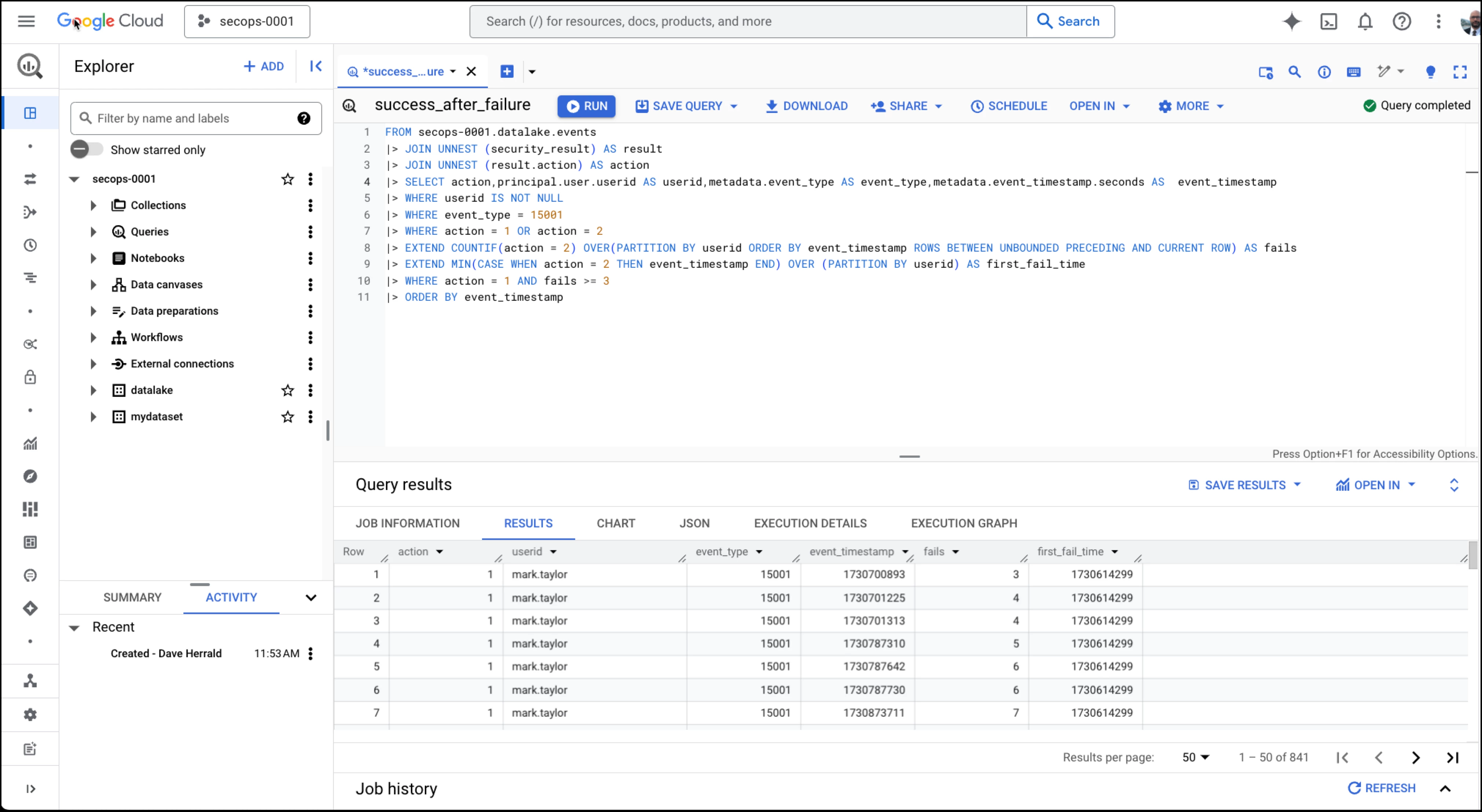
Many consider this example the canonical use case for security information and event management (SIEM) tools. The query detects instances where an attacker attempts to log in using brute force or password-stuffing techniques. I included it here for a couple of reasons. First, I want to show that pipe syntax is well-suited to perform traditional SIEM-style detection queries, and second, I want to show the power of SQL window functions and how they work in the |> EXTEND operator. For those familiar with SPL, note how window functions offer similar capabilities to the "streamstats" and "eventstats" commands. In this example, window functions allow us to look back at recent events to identify streaks of failed logins followed by a successful login. Each row in the final output of this query represents a detection.
Example - Multiple Failed Logins Followed by a Successful Login
| Pipe Syntax Query, line-by-line | Explanation | |
| 1 | FROM `secops-0001.datalake.events` | Bootstrap the query using a standalone "FROM" clause with the events table. |
| 2 | |> JOIN UNNEST (security_result) AS result | In UDM, security_result is a repeated field. Repeated UDM fields become array columns in BigQuery during the export process. |> JOIN UNNEST is a quick way to flatten this array for further processing. There are other ways to deal with this necessary evil in our schema. We show another approach in our next example. |
| 3 | |> JOIN UNNEST (result.action) AS action | More flattening! |
| 4 | |> SELECT action, | Indicate a few columns (UDM fields) of interest and give them convenient names. |
| 5 | |> WHERE userid IS NOT NULL | This dataset has many events with no userid. Here, we filter them out. |
| 6 | |> WHERE event_type = 15001 | Filter for only user login events. 15001 represents USER_LOGIN in the UDM enumerated type. |
| 7 | |> WHERE action = 1 OR action = 2 | Filter for only successful and blocked user logins, represented by 1 and 2 in the UDM enumeration, respectively. |
| 8 | |> EXTEND | This is the most complicated and powerful pipe syntax operator we've seen so far. Recall the |> EXTEND operator adds a new column to the output. We name the new column "fails," which will hold a count of recent failed logins (indicated by action=2) for this user. This analysis requires us to look at previous events (rows in the table) using a SQL window function. That “ROWS BETWEEN UNBOUNDED PRECEDING AND CURRENT ROW” incantation is the frame clause for the SQL window function. It describes how far back the window function should look during its analysis. Describing it in detail is beyond the scope of this blog, but it is a reminder that Google SQL is a powerful query language with many useful features! |
| 9 | |> EXTEND | Here, we use another window function to determine the date/time stamp of this user's first failure in the streak and capture it in a new column named "first_fail_time." |
| 10 | |> WHERE action = 1 AND fails >= 3 | With the complicated analysis done in the |> EXTEND operator and window functions above, here we apply a static threshold to implement the rule logic of “multiple (3 or more) failed logins followed by a successful login.” Each row of the final output table represents a “detection.” |
| 11 | |> ORDER BY event_timestamp | Sort the rows in chronological order, which we interpret as "detections" in this example. |
Example - Enriching Data Using Joins
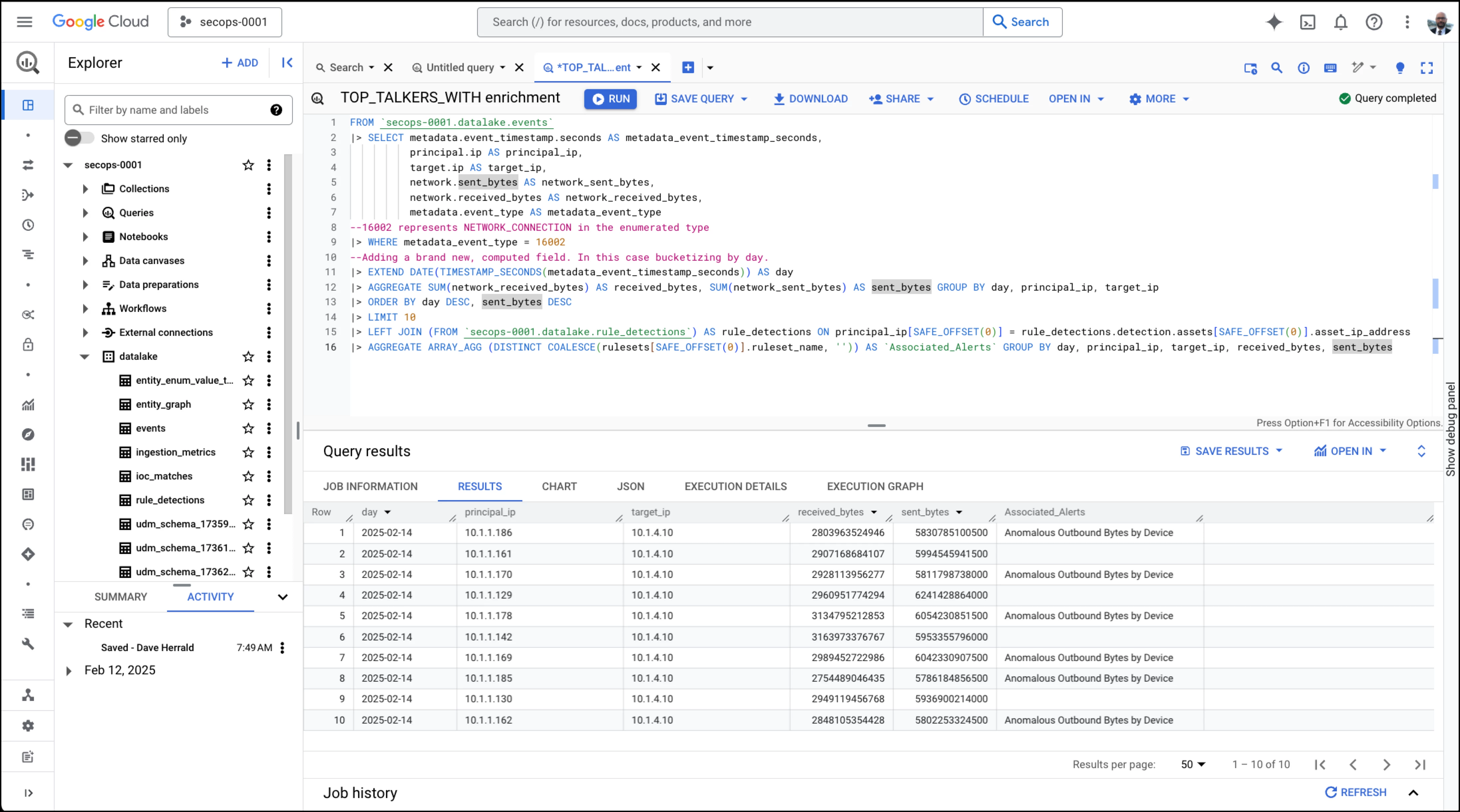
In this example, we'll further show how to use joins in pipe syntax to enrich results from a query with data from a different BigQuery table. We'll build on the Top Talkers example to determine whether the principal (source) IP address in any of our Top Talker pairs has been involved in any detections captured by Google SecOps. This additional context might help an analyst determine if the observed level of traffic is normal or anomalous. This example also shows some practical pipe syntax and Google SQL techniques I use often. For starters, the linear nature of pipe syntax allows us to take a helpful query, the top Talker example, and extend the query by adding more operators to the end. It's a common technique in flow-based query languages, and pipe syntax makes it easy to do in Google SQL. We'll also use indexes to demonstrate another way to deal with the arrays that are prevalent in the UDM-based schema exported from Google SecOps. The results show that Google SecOps has identified several of our Top Talkers transmitting anomalous amounts of data.
Example - Enriching Data Using Joins
| Pipe Syntax Query, line-by-line | Explanation | |
| 1 | FROM `secops-0001.datalake.events` | Start with the Top Talkers example. |
| 2 | |> SELECT metadata.event_timestamp.seconds | |
| 3 | principal.ip AS source_ip, | |
| 4 | target.ip AS destination_ip, | |
| 5 | network.sent_bytes AS sent_bytes, | |
| 6 | network.received_bytes AS received_bytes, | |
| 7 | metadata.event_type AS event_type | |
| 8 | --16002 represents NETWORK_CONNECTION | |
| 9 | |> WHERE event_type = 16002 | |
| 10 | --Adding computed column. | |
| 11 | |> EXTEND DATE(TIMESTAMP_SECONDS(timestamp_seconds)) | |
| 12 | |> AGGREGATE SUM(received_bytes) AS received_bytes, | |
| 13 | |> ORDER BY day DESC, sent_bytes DESC | |
| 14 | |> LIMIT 10 | |
| 15 | |> LEFT JOIN ( | Use the |> JOIN pipe operator to look up detections that our IP addresses may be involved with. We'll join our results with the "rule_detections" table, exported from Google SecOps, alongside the events table. We want to enrich our data based on the "principal_ip" column from our query, which matches the IP address from the asset in the rule_detections table. Note that instead of flattening the array in UNNEST ( as in previous examples), we access the first element using SAFE_OFFSET. |
| 16 | |> AGGREGATE | Finally, we use an additional |> AGGREGATE operator to gather the names of any alerts that the source IP is associated with. |
Note that while this example helps show how joins work in pipe syntax, the query is not ready for production. I'd improve it by joining on both principal IP and target IP and correlating on date/time. I'd also include more columns from the "rule_detections" table in the final output, like risk scores.
Wrapping Up
Pipe syntax for Google SQL is a powerful innovation that will make it much easier for security analysts familiar with pipe-delimited flow-based languages to get comfortable with powerful data platforms like BigQuery more quickly. It offers linear, logical flow and results in explainable SQL queries that are easy to understand, troubleshoot, and build upon. Ultimately, pipe syntax is still Google SQL and enjoys the same optimization and declarative semantics as all queries do. Pipe syntax is an enabler that brings security analysts closer to other analytic ecosystems and workloads. I hope to share more (and more advanced) security analytic use cases using Google SQL pipe syntax soon.