

Author: Robert Parker, Senior Technical Solutions Consultant
Co-Author: Domnic Chua, Global Security Architect
An Adoption Guide In Depth Review for Entity Relationship Graphs
In the contemporary threat landscape, static indicator analysis is no longer sufficient to track sophisticated adversaries who utilize ephemeral infrastructure and modular attack chains. Visual relationship mapping is the superior methodology for identifying the "connective tissue" between command-and-control (C2) domains, recycled malware variants, and pivot IP addresses (Get started with Threat Graph). The Google Threat Intelligence Graph transforms isolated data points into a cohesive narrative, allowing analysts to visualize the lifecycle of a campaign rather than just its individual symptoms (Overview).
The Google Threat Intelligence Threat Graph is a sophisticated engine built upon a massive dataset of files, URLs, domains, and IP addresses. Strategically, this tool shifts the security operations center (SOC) from a reactive search posture to proactive, relationship-oriented pivoting. By mapping over 30 distinct relationship types including downloaded files, parental execution chains, and domain-to-IP resolutions over time this enables analysts to move beyond the "what" of a threat to the "who" and "how," for footprinting the entirety of an adversary’s operational infrastructure. This Adoption Guide provides the framework for initializing investigations, mastering node interpretation, and executing advanced commonality hunting to achieve a comprehensive understanding of the tools and how to harness the power of visual threat graphs.
The modern cybersecurity landscape requires analysts to move beyond isolated indicators of compromise (IoCs) and understand the complex, interconnected ecosystems of digital threats. Google Threat Intelligence Threat Graph provides advanced visualization and relational analysis tools built on top of one of the world's largest security datasets.
What You Can Do With It:
-
Visualize Relationships: Transform flat lists of IoCs into interactive maps detailing over 30 types of relationships between the entities in your investigations.
-
Pivot Intelligently: Seamlessly traverse from a single malicious artifact (like a phishing URL or an undetected malware hash) to uncover an adversary's wider network of domains, IPs, and command-and-control (C2) servers.
-
Identify Threat Commonalities: Automatically analyze a cluster of nodes to extract shared characteristics (e.g., identical SSL certificates, shared Imphashes, or common hosting providers), turning isolated clues into robust YARA rules or blocklists.
Learning the Threat Graph Architecture: Nodes and Entities
Understanding "Node Anatomy" is critical for rapid triage during incident response. Visual markers serve as pre-cognitive indicators, allowing an analyst to assess the weight and severity of a threat before performing deep-dive forensics. This immediate situational awareness ensures that the investigation focuses on high-impact pivots rather than low-value artifacts.
Entity Type Classification
The following table defines the primary entities encountered within the Google Threat Intelligence environment and their visual icons:
| Entity Type | Visual Representation | Strategic Significance |
| Files |
| These are represented as rectangular nodes containing a file type icon (e.g., EXE, DLL, DOC). This visual cue allows analysts to instantly distinguish between executables, documents, and scripts within a complex infection chain. |
| Domains |
 Uses Favicon | Represented by the domain's favicon, if available. This is a powerful visual aid, as it allows analysts to spot brand impersonation (e.g., a fake PayPal icon on a strange domain) instantly. |
| URLs |

| Depicted by a specific icon (typically a globe or link symbol), differentiating specific web pages from the root domains they reside on. |
| IP Addresses |

| These nodes display the flag of the country where the IP is geo-located. If the country is undetermined, a black rectangle is used. This allows for immediate geographic profiling of infrastructure. |
| Relationship Nodes |
 
| Represented as circles containing a representative icon. These nodes are unique as they act as aggregators, grouping multiple entities that share a specific relationship type (e.g., "Contacted URLs") to prevent graph clutter. |
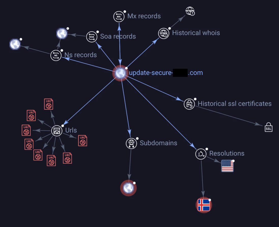
A sample illustration of the common icons used in Threat Graph
Advanced Node Analysis
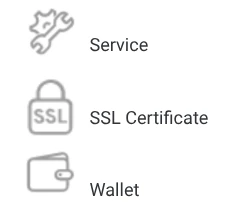
Organizations utilizing Private Graph features gain access to Advanced Node Types, which provide a "So What?" layer beyond standard public telemetry (Nodes).
-
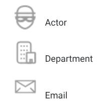
Targeting & Attribution: Nodes such as Actor, Victim, Department, and Email allow analysts to map specific victims within a corporate hierarchy and link them to known threat actors.
-
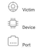
Infrastructure Depth: Device, Port, and Service nodes reveal the technical specifications of a target environment.
-
Infrastructure Persistence: The SSL Certificate node is a vital pivot point for identifying shared hosting environments, enabling analysts to track an adversary even after they migrate IP addresses.
-
Monetization Tracking: The Wallet node allows for the mapping of an adversary’s monetization infrastructure, potentially linking disparate malware campaigns to the same financial threat actor.
|
| 
|
|
A sample of manually Added Relationships which can be added to Threat Graphs
Interpreting Visual Logic: Verdicts and Relationships
Node Status and Navigation Indicators
Threat Graph utilizes a "Relationships Oriented" philosophy to reveal the movement of an adversary. This logic is communicated through color-coded telemetry, which is essential for rapid triage and identifying "known-bad" infrastructure during active incident response.
Color Coding and Visual Cues
| Visual Indicator | Visual Representation | Description & Significance |
| Red Nodes & Edges | 
| Indicate that the entity has one or more malicious detections from security vendors. |
| Gray/Black Nodes |
 | Indicate undetected entities or entities with zero detections. |
| Blue Nodes & Edges |

| Indicate the currently selected node and its direct connections. When a node is selected, its direct connections are highlighted, focusing the analyst’s attention on the immediate neighborhood of the threat. |
| Black Circles (Top Right) |

| A small black circle on a node means it has not been expanded yet. Double-clicking it will auto-expand its relationships. This signals that further relationships exist "behind" the node. Double-clicking triggers an auto-expansion to uncover hidden infrastructure. |
This icon distinction allows analysts to instantly separate verified threats from "gray-ware" or clean services. By tracing the paths between Red nodes, an analyst can map the core malicious spine of an attack.
Relationship Logic and Edge Directionality
Arcs represent the directional flow of a relationship (For example, a file contacted a specific IP or a file is executed by a parent file).
Google Threat Intelligence maps 30+ inter-item links, such as communicating_files, contacted_domains, and execution_parents. Directional lines represent the relationship between entities, therefore understanding the edges and the relationships helps us to answer various questions an intelligence analyst may have as they perform their investigations.
| Relationship | Direction | Investigative Question to Answer |
| Execution Parents | Backward | "How did this malware arrive?" |
| Dropped Files | Forward | "What did this malware install?" |
| Communicating Files | Lateral | "Who else uses this C2 server?" |
| Passive DNS | Historical | "What domains lived on this IP?" |
Scenario #1: Investigating an Emotet Infection
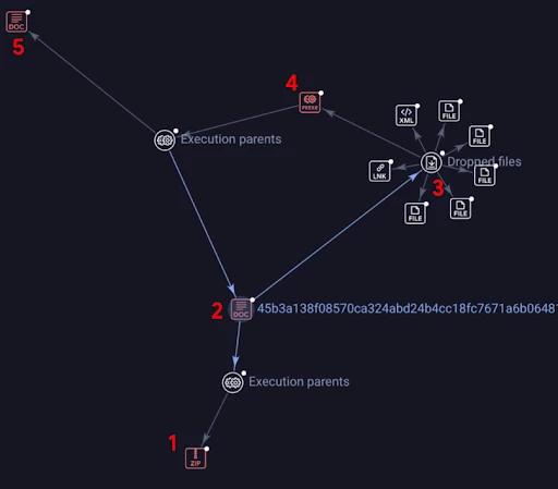
Threat Graph can help answer where did this malware arrive, what was its payload, and what other files also deliver this malware payload?
Follow along with the above Emotet infection example to understand how we can answer some of the above questions with regards to reviewing a malicious zip file and its contents of an Emotet related Word Document. In this scenario, imagine a user was sent a zip file as an email attachment. Within that zip file, is a malicious word document which contains Emotet malware.
-
We start with examining a Zip file at the bottom of the graph. This is the beginning of the infection chain, where a user was emailed a zip file as an attachment.
-
When looking at #2 on the graph, we see that is a malicious word document, which has an execution parent of #1, (the zip file). We follow the arrows from #2 to item #1, which tells us that this word document has an execution parent source of the zip file.
-
Reviewing the files around #3 we can now see these are the dropped files that came from the word document in #2. We can observe XML, LNK, and EXE files being dropped from the word document.
-
A portable executable PEEXE file is also dropped by the word document in #2. This is shown by the item #4. While this was initially clumped together by the other files in #3, this was moved away from the cluster for easier identification.
-
When asking the question, “What other word documents also execute this same EXE as #4, we see the additional file of #5 from the relationships perspective.
Instantiating and Managing Persistent Investigations
Threat hunting is an iterative, collaborative process. The ability to instantiate a persistent investigation ensures that findings can be saved, resumed, and peer-reviewed without loss of context.
Workflow Initialization
Investigations are typically started through two methods:
-
Direct Search: Use the search functionality to find public graphs, team-specific graphs, or specific hashes to identify existing investigations.

Searching for publicly shared threat graphs from the main page
-
The Pivot: From a standard file, domain or URL report, select More > Explore in Threat Graph to transition from static data into the visual synthesis engine (Get started with Threat Graph).
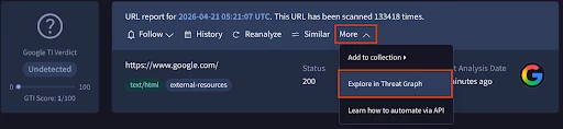
Pivoting from a search for a URL instantly into Threat Graph
Graph Management and Role-Based Access
Understanding RBAC for graphs is essentially for proper sharing and maintaining operational security. Access and modification rights are governed by three primary roles to maintain data integrity.
| Role | Permissions | When to Use |
| Owner | Full access; can delete the graph. | Ultimate control over the investigation lifecycle |
| Editor | Can expand/delete nodes; add collaborators. | Enables collaborative hunting and active peer review |
| Viewer | Read-only access. | Ideal for sharing finished intelligence with stakeholders without risking data modification |
Privacy and Operational Security (OPSEC) Considerations
Visibility settings are critical for maintaining the confidentiality of an ongoing investigation.
-
Private Status indicates Saved investigations are private by default, ensuring that only authorized team members can view the graph.
-
Public/Embed Status means once an investigation is finalized, it can be set to public or embedded into external reports using iframes. This facilitates broader community intelligence sharing.
Advanced Analytical Actions: Node Expansion and Submissions
Pivoting is the force multiplier of threat intelligence. By expanding nodes, an analyst uncovers the "unseen" connections that an adversary believes are obscured.
Expansion Mechanics and Tactical Outcomes
-
Using the full expansion option triggers all available expansions for a node simultaneously. This can be performed by selecting the full expansion Icon, or double clicking the node in the graph. This is used to rapidly footprint a campaign’s initial scope, but also can lead to a very confusing and busy graph.
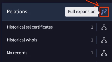
Full expansion triggers all the relationships to be shown at once, however this can make for a messy, and visually difficult to follow graph
-
It is recommended to start with a specific pivot which attempts to answer hypotheses, and in doing so uses a simple targeted expansion. Remember our hypothetical questions from earlier, expand the relations out one at a time to answer your hypotheses during an investigation.
-
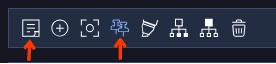
A targeted expansion is a manual selection of specific links to prevent "graph clutter" in high-volume environments. This systematic approach helps us to answer our questions about the entity to build & understand the relationships of the entity in question. Those Icons are the ones shown below.
Expanding on the single relationship at a time button
- Visual Noise Reduction (Highlighting): The Highlight feature hides all nodes not directly connected to a selected entity. This is vital in complex graphs to maintain focus on the relevant attack path.
Interactive Layout Controls
To create a readable narrative of an attack, analysts should utilize the following controls:
-
Labeling: Allows for custom naming of nodes (e.g., "Primary C2") to provide clarity for other collaborators
-
Pinning: Removes the "gravity" or animation from the graph, sticking a node to a specific location.
Labeling (Left Icon) and Pinning (Right Icon)
Temporal and Geographical Context
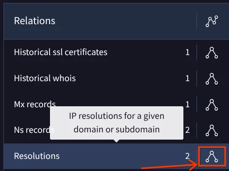
The Submission Box on the left hand navigation panel provides a graphical representation of when and where a file was seen. By grouping submissions by country or upload date, analysts can identify the origin of a campaign and the adversary's target demographic over time (Nodes).
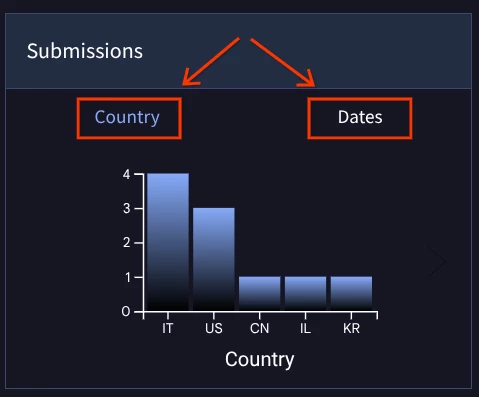
Viewing which countries have submitted the file and when the file was uploaded
Executing Commonality Calculations and Hunting
Pattern recognition is the hallmark of a master hunter. Adversaries often reuse SSL certificates, file paths, or registration details across disparate attacks. Commonality calculations allow analysts to identify these shared TTPs in real-time.
Advanced Tools: Commonalities Workflow
Calculations are performed based on the current selection in the right-side toolbar.
The calculate commonalities button
-
Global Pattern Check: If 0 or 1 node is selected, the toolbar shows commonalities for the entire graph, enabling an analyst to find broad themes across the whole investigation.
-
Selection Analysis: If more than 1 node is selected (via Shift + Click or Drag), the toolbar calculates commonalities specific to those items.
-
Manual Trigger: For a Relationship Node, click Calculate commonalities in the left drawer to analyze all "children" grouped under that node.
Advanced Tools: Similarity with Vhash and Similar-to:
To elevate an investigation from simple analysis to proactive threat hunting, analysts must utilize GTI's advanced processing engines.
The Commonalities Engine: By selecting a cluster of malicious files or infrastructure and clicking "Calculate Commonalities", the platform automatically finds shared metadata and behaviors. This is critical for zero-day hunting. For example, if two separate malicious Word documents share the same specific Office Macro Name or Exiftool Language Code, you can pivot on those commonalities to find related, undetected infrastructure.
Vhash vs. Similar-To vs ssdeep functionality:
-
Vhash: A proprietary similarity clustering algorithm created by GTI based on simple structural features. Searching via vhash:<vhashvalue> yields an Exact Match of a structural blueprint, useful for pinpointing the exact same malware builder or document template.
-
Similar-to: Searching via similar-to:<SHA-256> calculates algorithmic distance (a fuzzy match). This is ideal for discovering evolving malware variants, slightly modified payloads, or broader threat families. This is used by searching for this in the Google Threat Intelligence Search bar.
-
ssdeep: a standardized, open-source fuzzy hashing algorithm, which Unlike a traditional cryptographic hash (like MD5 or SHA256) that completely changes if a single byte is altered, ssdeep breaks a file down into smaller chunks, hashes those individual chunks, and combines them. This allows you to compare two files at the byte-content level and get a mathematical percentage of how similar they are (e.g., an 85% match), even if a threat actor added, removed, or modified parts of the payload. ssdeep is an open-source standard, whereas vhash and similar-to: are proprietary to Google Threat Intelligence.
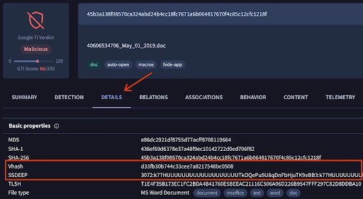
How to review the Vhash and ssdeep of a file hash using our Word Document from Scenario #1
Moving from Visualization to Active Defense
Identified commonalities can be operationalized via the contextual menu (Commonalities and Hunting):
-
Launch VT Search: Find other entities in the global database sharing this attribute (Commonalities and Hunting).
-
Add Relationship Node: Visually link all nodes sharing the commonality on the graph (Commonalities and Hunting).
-
Create YARA Rule: Automatically generate a YARA ruleset based on the shared attribute. This bridges the gap between investigation and active detection.
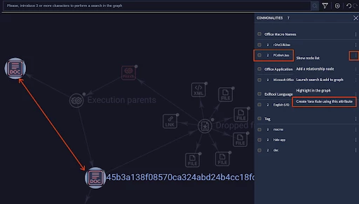
Creating a YARA rule for Livehunting using the common macros found in both Word documents from Scenario #1.
Practical Incident Response Scenarios
Below are real-world examples illustrating how to use Threat Graph during an incident response or threat hunting engagement.
Practical Use Case 1: Unmasking a Massive Phishing Network (Infrastructure Reuse)
Threat Scenario:
An analyst investigated a suspicious WhatsApp link targeting users of "Yad2" (a legitimate secondhand marketplace).
The Pivot:
-
The analyst dropped the initial phishing URL into Threat Graph, which revealed the specific IP address hosting the site.
-
Knowing that attackers rarely buy a new server for every single site, the analyst pivoted on that IP address node to view all domains resolving to it.
The Result:
The single WhatsApp link was actually part of a massive, global operation. The graph revealed over 800 different scam domains hosted on that exact same infrastructure, impersonating hundreds of legitimate global brands.
Practical Use Case 2: Mapping the Infection Chain & Spotting Decoys (Agent Tesla)
Threat Scenario:
A suspicious .exe downloader was found on an endpoint. The analyst needed to know what the payload was and how it got there.
The Pivot:
-
Graphing the executable hash revealed its "Parents" (the RAR archives the executable was initially embedded inside).
-
Expanding the "Communicating Domains" from the executable revealed the malware was reaching out to several benign football club sites including realmadrid[.]com, chelseafc[.]com) alongside a highly suspicious, randomized domain.
The Result:
The visual layout made it immediately obvious that the football domains were "red herrings" meant to confuse automated sandboxes and analysts. By pivoting strictly on the suspicious domain and checking its "Downloaded Files", the analyst found the true final payload of the Agent Tesla infostealer.
Practical Use Case 3: Containing the "Blast Radius" in Incident Response
Threat Scenario:
A company's SIEM alerts on a zero-day exploit payload executing on a single employee's laptop. The immediate instinct is to wipe the laptop, but the SOC needs to know if the attacker spread laterally.
The Pivot:
-
The responder graphs the initial payload hash and pivots to find its C2 IP address.
-
They pivot on that C2 IP, revealing 5 other distinct malware hashes communicating with that same server.
The Result:
The responder takes those 5 new, undiscovered hashes and queries their internal EDR (Endpoint Detection and Response) tool. They find that 3 other laptops in the marketing department have those sibling hashes quietly running on them. VT Graph allowed them to find the full scope of the breach rather than just playing whack-a-mole with the first alert.
Operationalizing and Disseminating Findings
A graph investigation is only valuable if it leads to defensive action. Once you have mapped a threat ecosystem, you must operationalize it:
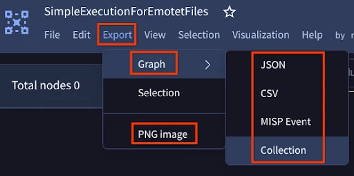
Exporting your Threat Graph findings
-
Export to Defensive Controls: Using the Export menu, you can download graph nodes as JSON, CSV, or STIX formats, or export them directly as a MISP event to feed into your SIEM (SecOps/Splunk) or EDR blocklists.
-
Send to Collections: Export the entities from your Threat Graph into a Collection inside of Google Threat Intelligence which can be shared with your team, or integrated into your IOC Stream data.
-
Convert to Detections: Use the Commonalities function to identify shared behaviors (e.g., common Office Macro names), and convert these patterns into automated YARA rules via Livehunt to catch future zero-day variants.
-
Collaborate via Private Graphs: Save your investigation as a Private Graph to keep your ongoing incident response confidential. You can add specific SOC team members as Viewers or Editors, allowing synchronous collaboration without leaking sensitive data to the public Google Threat Intelligence community.
-
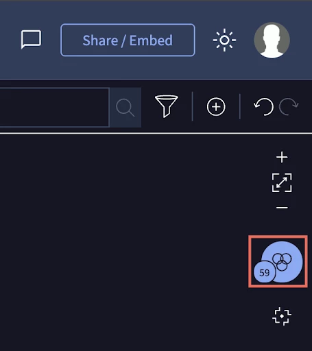
Executive Reporting: Use the Embed feature to copy HTML snippets of your graph directly into incident tickets or executive threat intelligence briefings.
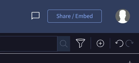
Locating the share / embedding link For Threat Graphs
Summary and Path to Mastery
The transition from tool user to master hunter requires seeing the Threat Graph as a synthesis engine for the entire Google Threat Intelligence ecosystem. Professional rigor demands a systematic approach to every investigation, moving beyond isolated indicators to understand the complex, interconnected ecosystems of digital threats. By leveraging over 30 distinct relationship types, analysts can move beyond the "what" of a threat to footprint the "who" and "how" of an adversary’s operational infrastructure. This strategic shift transforms the SOC from a reactive search posture to one of proactive, relationship-oriented pivoting and visual campaign mapping.
Strategic Checklist for Success
-
Resolve Unexpanded Nodes: Always check for the "black circle" indicators to ensure no part of the adversary's infrastructure remains hidden.
-
Triage via Verdicts: Prioritize Red-verdict nodes during the initial pivot phase to identify the core malicious infrastructure.
-
Regularly Calculate Commonalities: Use global pattern checks to find the "pivot points" that link isolated incidents to wider campaign activity.
-
Leverage External Context: Utilize the Global Landscape module to compare internal graph findings with established Threat Profiles, Actors, and Malware Families to achieve accurate attribution.