

Written by: Christopher Galbraith, Megan DeBlois, Phil Tully
Security has long been a cat and mouse game of what we know about an adversary and how they go about evading our sights—be it infrastructure they use in their operations; tactics, techniques, and procedures (TTPs); or even the type of targets they are after. The constantly evolving threat landscape (along with the sheer volume of threat intelligence data) makes it difficult for security teams to assess and monitor the most relevant threats to their organizations. The Google CloudSec Data Science team released this blog post to accompany our recent CAMLIS presentation illustrating how we can ease this burden through machine learning. By using this approach we are dramatically shifting the paradigm to give defenders the advantage, helping them focus on the most likely threats based on signals from Google and Mandiant expertise.
Background: Customer Threat Profiles
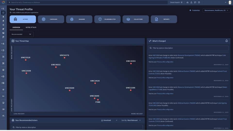
Earlier this year at RSA we launched Google Threat Intelligence, combining diverse sets of threat intelligence sources with Mandiant frontline expertise, VirusTotal community intelligence and threat insights from Google in a single product. The result is a new era of unparalleled visibility of threats across the globe. There are billions of observables in Google Threat Intelligence—including the world’s largest malware database from VirusTotal with over 50 billion files and Mandiant’s frontline threat intelligence fueled by over 400 incident investigation hours in 2023. With so much visibility, prioritization of threats becomes key to unlocking proactive security outcomes for threat hunting, security control assessment, strategic risk management and more. For this reason we introduced in-product threat profiles that produce automated, real-time, machine learning-driven recommendations of the most relevant threats to your organization.
The threat profile is intended to identify threats that are most relevant to an organization based on various dimensions like its industry, location of operation, and cybersecurity interests including motivations of threat actors, malware roles and threat source locations. It leverages insights from past incident data, intelligence information, and observations in peer organizations or regionally focused activity. The threat profile helps an organization not only understand the threats that matter most, but informs security detection prioritization, highlights gaps, trends and patterns, and can help guide security policies and strategic resource allocation. When communicated in a timely manner, the threat profile provides decision makers comprehensive situational awareness, and aids the overall cyber defense organization in prioritizing, coordinating, and taking appropriate actions based on a common threat picture.
To create a threat profile, users can configure one or more operating locations, industry verticals, and threat characteristics of interest including actor motivations, malware roles and threat source locations. The ML model then recommends the most relevant threat intelligence objects for these personalized interests learned from Mandiant’s frontline intelligence data and expert knowledge.
 Learn more about threat profiles within Google Threat Intelligence.
A Metric Learning Approach to Populating Threat Profiles
Introduction
Threat intelligence data is massively heterogeneous and highly interconnected. For example, threat actors have relationships to particular malware families they tend to use, which in turn have relationships to the vulnerabilities they exploit. These basic relations can be further derived for more complex semantics. To enable access to the information needed for analysts to do their day jobs, threat intelligence data is typically stored as heterogeneous graphs. However, making this information actionable requires numerous manual pivots, complex queries, and validation/testing at each step of the process.
Many industrial applications of machine learning are concerned with data having different modalities or feature distributions. Heterogeneous graphs offer a unified view of these multimodal systems by defining multiple types of nodes for each object type (each with their own attributes with differing feature distributions) and edges for the relationships between them. A common task for heterogeneous graphs is learning node embeddings for use in downstream applications like information retrieval, clustering, and as features in other models. In particular, heterogeneous graph representation learning approaches have been applied to learning latent representations of users for personalized recommendation in social networking e1], search ]2], a3], travel ]4], and retail n5].
Our motivation for this feature was simple—how can we quickly get actionable insights into security practitioners’ hands without them having to go through this arduous process? We drew inspiration for our approach from latent user representation methods for personalized recommendation. We treat organizations as “users” and leverage the relationships and features from a threat intelligence heterogeneous graph to jointly learn embeddings of both organizations and threat intelligence objects. Figure 1 illustrates the basic concept behind this approach. In this blog post, we will focus on the methodology used to learn the embeddings and how these embeddings can be used to populate threat profiles.
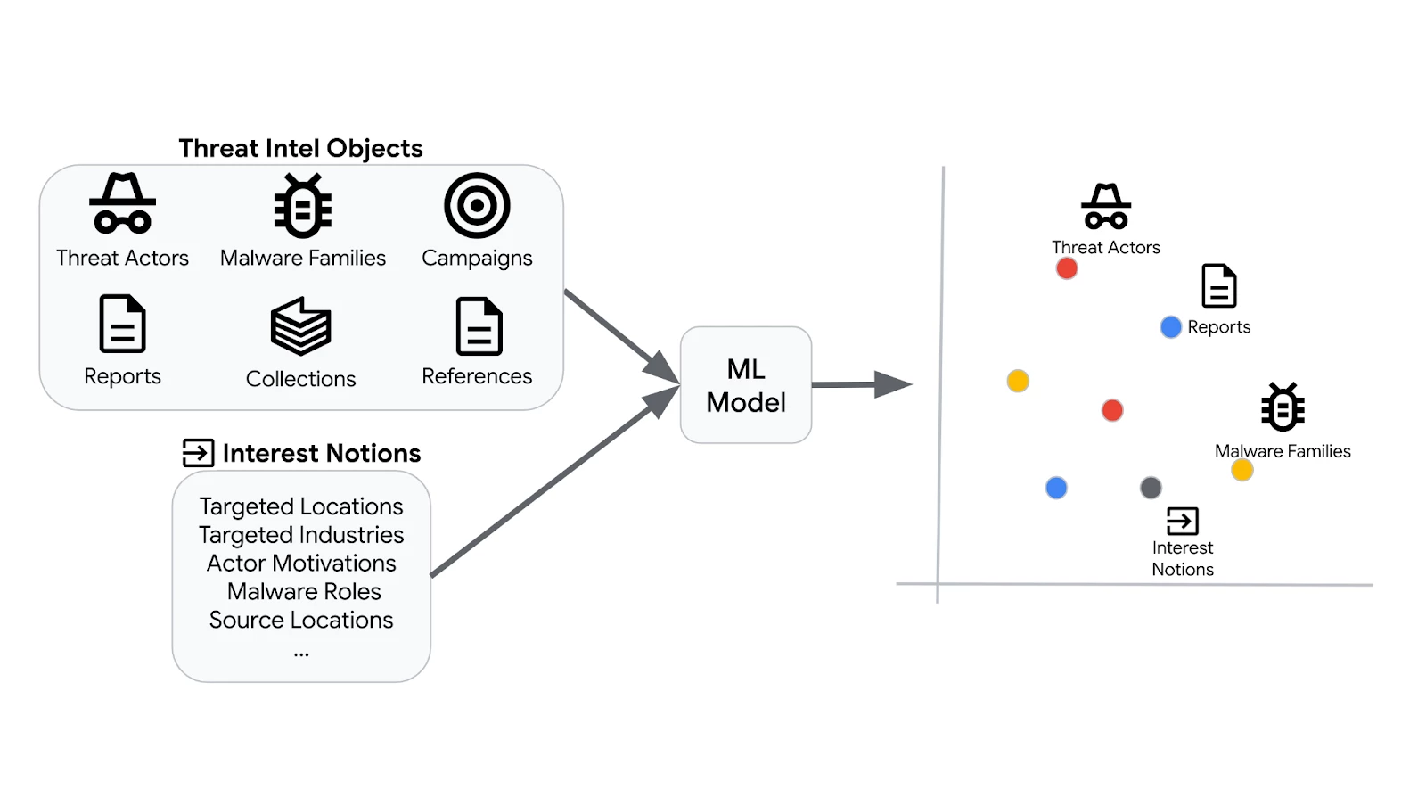
 Figure 1: (Top) Basic concept behind heterogeneous object embeddings for threat intelligence data. (Bottom) Recommending threat intelligence objects based on nearest neighbor distances to the interest notions embedding in the learned embedding space.
Methodology
We leveraged a triplet network to produce threat intelligence embeddings. Triplet networks are self-supervised metric learning models that rank positive (or similar) and negative (or dissimilar) samples based on an anchor object. The model produces embeddings for all three objects (anchor, positive, and negative) via parallel neural networks with shared weights. The triplet loss objective function seeks to minimize the distance in the embedding space between the anchor and positive samples while maximizing the distance between the anchor and negative samples as shown in Figure 2.
 Figure 2: Triplet loss in action. The model learns to embed the anchor and positive (or similar) objects closer together than the anchor and negative (or dissimilar) objects.
The parallel networks used in the triplet model for generating embeddings of threat intelligence objects are set-based neural network encoders. We treat each object feature as a set of discrete values, encode and combine them, and pass these representations through a sequence of hidden layers to obtain the object’s embedding. The features we used include a variety of information from demographics of previous attack history (e.g., industries/locations targeted) to how the threat intelligence object typically operates (e.g., vulnerabilities exploited, TTPs, impacted operating systems, etc).
The most critical element of the training setup is the construction of batches of triplets. Doing this well results in a learned embedding space that adheres to the semantics of the threat intelligence graph and reflects subject matter expertise. The batch sampling strategy we employed was the result of a feedback loop with subject matter experts. We iterated on model versions by assessing expert feedback on outputs and collaborating on strategies to move the embedding space in desired ways.
Training batches are constructed by sampling anchor objects of each threat intelligence type (e.g., threat actors, malware families, etc). Then, for every anchor object sampled and relationship type it appears in, we leverage the threat intelligence heterogeneous graph for selecting positive samples. Negative samples are taken to be objects that do not have a link in the graph (subject to constraints that were developed alongside subject matter experts). For example, if the anchor object is threat actor APT43 and the relationship type is {actor, malware family}, we would take all malware families confirmed to be used by APT43 as the positive samples and randomly sample malware families that have not been used by APT43 as negative samples. See Figure 3 for an illustration of the batch sampling algorithm.
 Figure 3: Batch sampling of triplets from the threat intelligence heterogeneous graph.
Results
We quantitatively evaluated our approach by a suite of metrics including entropy in recommended objects across various inputs to the model, “freshness” of the recommendations as measured by the last confirmed activity, and comparison against expert-crafted threat profiles created during customer engagements. See Table 1 for more details.
| Model | Entropy | Freshness - Average Age (days) | Frontline Actor Precision (%) | Frontline Malware Precision (%) |
| v2* | 1.84 | 32.88 | 36.31 | 20.43 |
| v3** | 3.10 | 30.70 | 37.75 | 20.87 |
Model evaluation metrics comparing two versions of the embeddings used for information retrieval. Entropy (higher is better) measures the variability of and Freshness (lower is better) measures the time since last confirmed activity in the recommended objects across multiple interest notions input to the system. Frontline precision of actor and malware recommendations measures the average agreement between model output and reports produced by Mandiant analysts during customer engagements (higher is better). Note that these reports include observed IOCs in customer environments, which are used to add actors and malware families. The models used to generate recommendations did not have access to this information.
*Training data pulled Q1 2024.
**Training data pulled Q3 2024.
Additionally, we have threat analysts perform thorough qualitative reviews on a monthly basis. This allows us to reassess how subject matter experts’ threat assessments evolve over time and tweak the model through feature engineering or by updating to the training regime to instill expert knowledge into the model on a continuous basis.
The end result is a system that produces the most relevant threat intelligence for a given set of interest notions as shown in Figure 4. We additionally generate explanations based on alignment with interest notions to foster transparency and trust in the system.
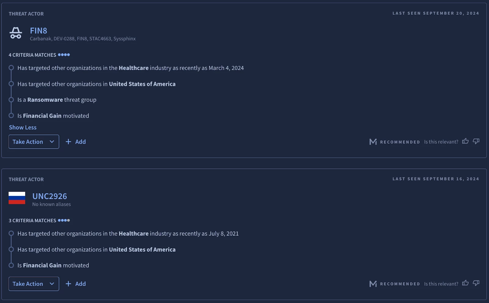
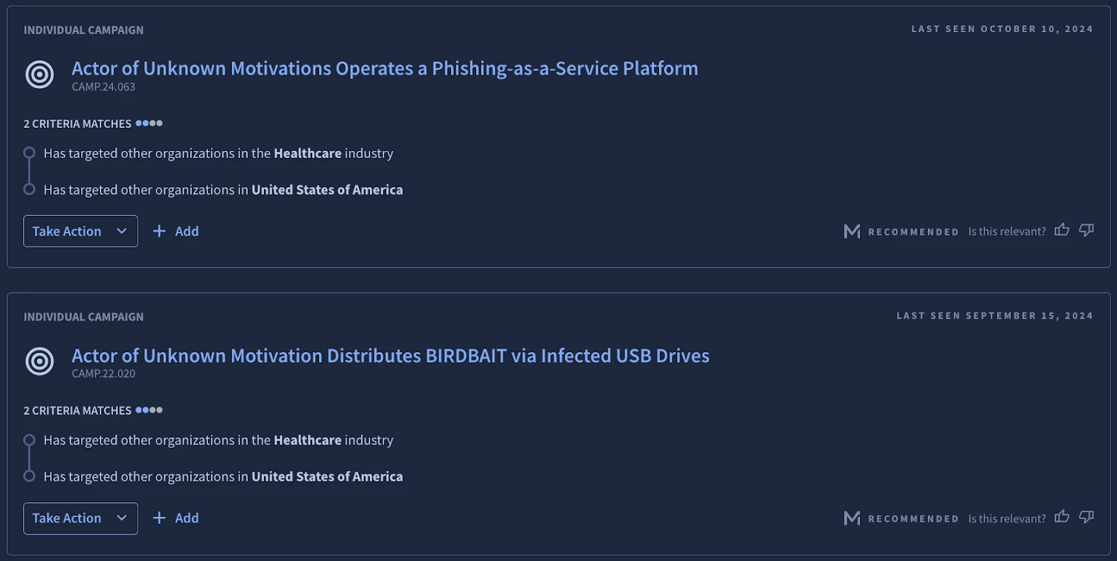
Figure 4: Example actor (top) and campaign (bottom) model recommendations in Google Threat Intelligence along with corresponding explanations underneath the “Criteria Matches” heading.
Conclusion
Google is transforming the industry with personalized threat intelligence that is a prerequisite for every proactive security program, giving customers a way to focus when surrounded by billions of indicators and artifacts. In this blog post, we introduced an ML-driven approach to recommend the most relevant threats to an organization. The CloudSec Data Science team will continue to incorporate high fidelity leading signals to make it easy for our customers to take action on the best and most relevant human curated, crowdsourced, and frontline threat intelligence on the planet. Stay tuned for future updates!
References
e1] A. Pal, C. Eksombatchai, Y. Zhou, B. Zhao, C. Rosenberg, and J. Leskovec. PinnerSage: multi-modal user embedding framework for recommendations at Pinterest. In KDD, 2020.
2] H. Cheng, L. Koc, J. Harmsen, T. Shaked, T. Chandra, H. Aradhye, G. Anderson, G. Corrado, W. Chai, M. Ispir, R. Anil, Z. Haque, L. Hong, V. Jain, X. Liu, and H. Shah. Wide & deep learning for recommender systems. In DLRS@RecSys, 2016.
23] P. Covington, J. Adams, and E. Sargin. Deep neural networks for Youtube recommendations. In RecSys, pp. 191–198, 2016.
,4] M. Grbovic and H. Cheng. Real-time personalization using embeddings for search ranking at AirBnb. In KDD, 2018.
,5] X. Zhao, R. Louca, D. Hu, and L. Hong. Learning item-interaction embeddings for user recommendations. 2018.