


In the previous two blogs in the New to Google Security Operations (SecOps) series, we’ve taken a look at building multi-stage searches in YARA-L to generate that “stat of a stat” result that we are often hunting for within our data sets.
In these blogs, the example searches contained a named stage and a root stage. The first blog focused on aggregating events and then outputting a result with a second aggregation. The second used a time window in the named stage to aggregate data.
This time, we are going to apply both of these concepts in a single multi-stage search. The search we will build will contain two named stages, followed by a root stage which will generate another statistical output that you can use in your analysis!
Z-score
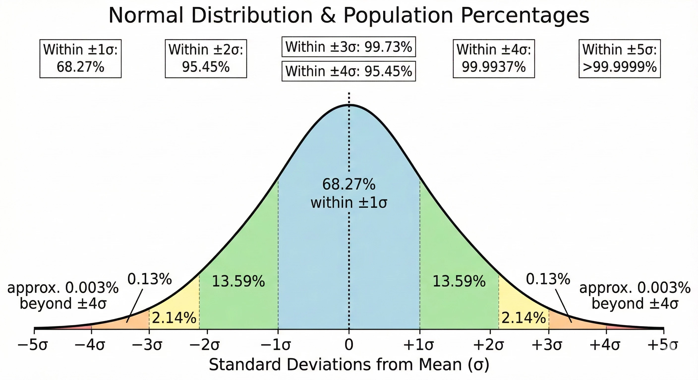
Our example today will focus on calculating a Z-score. A Z-score, sometimes referred to as a standard score, measures the number of standard deviations a data point is from the mean of a data set. That said, a Z-score assumes that the data being analyzed follows a normal distribution, often referred to as a Bell curve. From a cybersecurity perspective, a Z-score provides us the ability to identify outliers within our data set by identifying data above (or below) the average of that data. If the data is extremely bursty or prone to wild variances, a Z-score may not be the best statistical measure for your use case.
The formula to calculate a Z-score is:
z = (x - μ) / σ
To calculate it, we need the following:
- The data point of interest - x
- The mean (average) of the population - μ
- The standard deviation of the population - σ
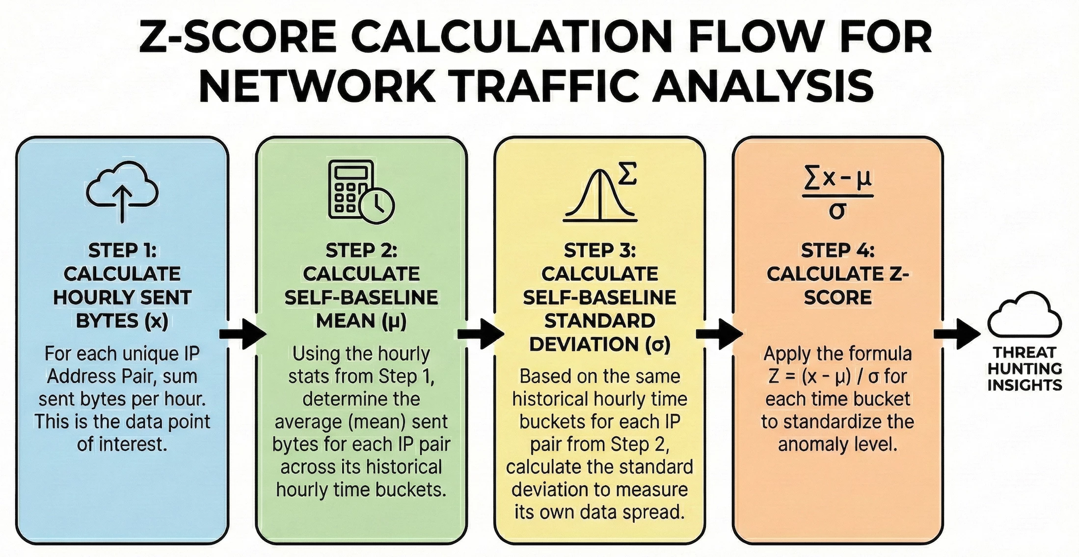
This type of search cannot be performed with a single pass across the data set. For this example, we are going to calculate a statistical value by creating hourly buckets of the sum of the sent bytes for each IP pair. We will then take that output and calculate both the mean and the standard deviation. Once we have those measures, we can put it all together to generate Z-scores for each hourly IP address pair.
The environment I’m using for this example contains a set of Windows systems with a Corelight sensor monitoring the traffic which is where we are getting the values in the network.sent_bytes field to calculate the Z-score. We are searching network traffic for a specific day between the hosts in our network to determine if we have any outlier traffic flows broken out by hour.
Step 1: Calculate the Hourly Sent Bytes
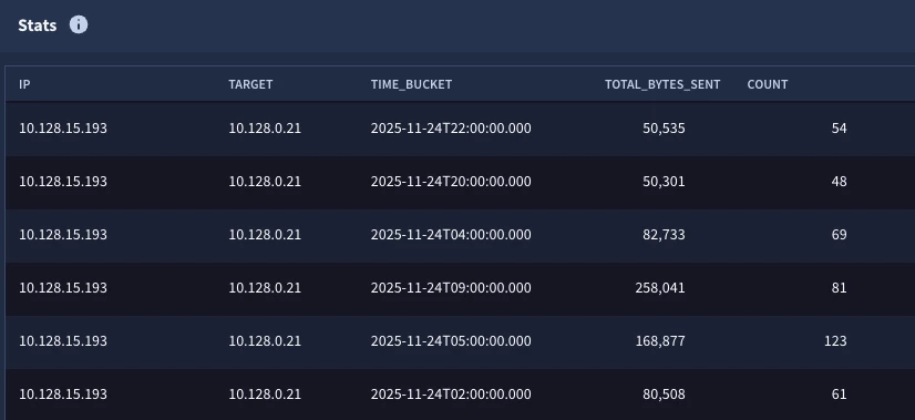
Let’s start by calculating the total sent bytes for each IP pair by hour. In the search below, we are narrowing the data set to just network connection events within our IP block. In the match section, we are aggregating the events by the principal and target IP addresses and the hourly time bucket, and in the outcome section we are calculating the sum of the bytes as well as generating a count of the number of events.
metadata.event_type = "NETWORK_CONNECTION"
net.ip_in_range_cidr(principal.ip, "10.128.0.0/16")
net.ip_in_range_cidr(target.ip, "10.128.0.0/16")
network.sent_bytes > 0
$ip = principal.ip
$target = target.ip
match:
  $ip, $target by hour
outcome:
  $total_bytes_sent = sum(cast.as_int(network.sent_bytes))
  $count = count(metadata.id)
The output will have five columns, one for each field referenced in the match and outcome sections. All of these columns can be leveraged in future stages of the search.
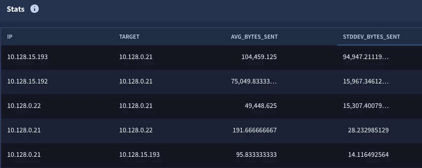
Steps 2 & 3: Calculate the Mean and Standard Deviation
These steps generate the “stat of a stat” that we’ve explored in the previous two blog posts. We have taken the initial statistical search from Step 1 and created a named stage called hourly_stats. To this we have added a root stage that is calculating the average and standard deviation.
stage hourly_stats {
metadata.event_type = "NETWORK_CONNECTION"
net.ip_in_range_cidr(principal.ip, "10.128.0.0/16")
net.ip_in_range_cidr(target.ip, "10.128.0.0/16")
network.sent_bytes > 0
$ip = principal.ip
$target = target.ip
match:
  $ip, $target by hour
outcome:
  $total_bytes_sent = sum(cast.as_int(network.sent_bytes))
  $count = count(metadata.id)
}
//root stage
$ip = $hourly_stats.ip
$target = $hourly_stats.target
match:
  $ip, $target
outcome:
  $avg_bytes_sent = window.avg($hourly_stats.total_bytes_sent)
  $stddev_bytes_sent = window.stddev($hourly_stats.total_bytes_sent)
When we execute our search, we can see that we have these statistical calculations for each IP pair. Notice we don’t have a time window in the results here. In this case, we want the average and standard deviation for the IP pairs, not the individual buckets.
Now that we have all three components required to calculate a Z-score for each time bucket, we can generate our output.
Step 4: Calculating Z-scores for IP Pairs and Time Buckets
We are going to take the logic from the previous search that we used to create the average and standard deviation calculations and convert this into its own stage named aggregate_stats. This named stage will need to be enclosed in curly brackets like the first stage we created.
stage hourly_stats {
metadata.event_type = "NETWORK_CONNECTION"
net.ip_in_range_cidr(principal.ip, "10.128.0.0/16")
net.ip_in_range_cidr(target.ip, "10.128.0.0/16")
network.sent_bytes > 0
$ip = principal.ip
$target = target.ip
match:
  $ip, $target by hour
outcome:
  $total_bytes_sent = sum(cast.as_int(network.sent_bytes))
  $count = count(metadata.id)
}
stage aggregate_stats {
$ip = $hourly_stats.ip
$target = $hourly_stats.target
match:
  $ip, $target
outcome:
  $avg_bytes_sent = window.avg($hourly_stats.total_bytes_sent)
  $stddev_bytes_sent = window.stddev($hourly_stats.total_bytes_sent)
}
//root stage
$aggregate_stats.ip = $hourly_stats.ip
$aggregate_stats.target = $hourly_stats.target
outcome:
  $ip = $hourly_stats.ip
  $target = $hourly_stats.target
  $hour_bucket = timestamp.get_timestamp($hourly_stats.window_start)
  $z_score = ($hourly_stats.total_bytes_sent -  $aggregate_stats.avg_bytes_sent)/$aggregate_stats.stddev_bytes_sent
  $events_per_pair = $hourly_stats.count
There are a couple of items in this search that I’d like to highlight:
- The two named stages are linked to the root using the IP address placeholder variables
- There is no additional aggregation required in the root stage, so there is no match section in the root
- The outcome section contains the columns that will be displayed
- The calculation for the Z-score is using values from both stages in it. Notice how we take the bytes from the hourly stats and then subtract the average from the aggregate and then divide that difference from the standard deviation (also from the aggregate).
When we run the search, we get the following.
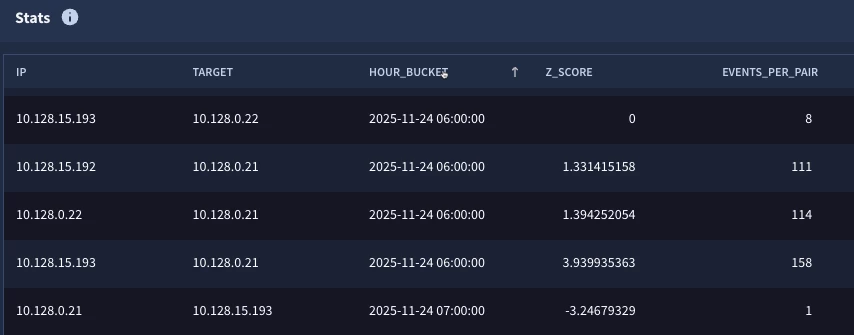
This is looking pretty good, but there are a few things we may want to do to improve our result set. To start with, IP pairs that have a very low event count may not be statistically significant for this specific use case. Second, if we are performing outlier analysis, perhaps I don’t want to see the Z-scores that are what we might consider normal. If you look at the bell curve, three standard deviations should cover 99.7% of the population, so perhaps we just want the events that are beyond three standard deviations. Finally, I’d like some additional context in my results. It would be helpful to include the average and standard deviation for the IP pairs as well. Let’s iterate on the search one more time to make these adjustments.
Tuning and Finalizing the Search
The previous root stage where we calculated the Z-score will become its own stage for this additional step. I went ahead and added the stage named z_score and curly brackets to this section.
stage hourly_stats {
metadata.event_type = "NETWORK_CONNECTION"
net.ip_in_range_cidr(principal.ip, "10.128.0.0/16")
net.ip_in_range_cidr(target.ip, "10.128.0.0/16")
network.sent_bytes > 0
$ip = principal.ip
$target = target.ip
match:
  $ip, $target by hour
outcome:
  $total_bytes_sent = sum(cast.as_int(network.sent_bytes))
  $count = count(metadata.id)
}
stage agg_stats {
$ip = $hourly_stats.ip
$target = $hourly_stats.target
match:
  $ip, $target
outcome:
  $avg_bytes_sent = window.avg($hourly_stats.total_bytes_sent)
  $stddev_bytes_sent = window.stddev($hourly_stats.total_bytes_sent)
}
stage z_score {
$agg_stats.ip = $hourly_stats.ip
$agg_stats.target = $hourly_stats.target
outcome:
  $ip = $hourly_stats.ip
  $target = $hourly_stats.target
  $hour_bucket = timestamp.get_timestamp($hourly_stats.window_start)
  $z_score = ($hourly_stats.total_bytes_sent - $agg_stats.avg_bytes_sent)/$agg_stats.stddev_bytes_sent
  $events_per_pair = $hourly_stats.count
}
//root stage
$z_score.ip = $agg_stats.ip
$z_score.target = $agg_stats.target
$z_score.z_score > 3.0 or $z_score.z_score < -3.0
$z_score.events_per_pair > 100
outcome:
  $ip = $z_score.ip
  $target = $z_score.target
  $hour_bucket = $z_score.hour_bucket
  $zscore = $z_score.z_score
  $events_per_pair = $z_score.events_per_pair
  $avg_bytes_sent = $agg_stats.avg_bytes_sent
  $stddev_bytes_sent = $agg_stats.stddev_bytes_sent
The new root stage has filtering criteria in it. Because we just want the outliers, we are going to specify that the Z-score must be greater than three or less than negative three. Because we don’t want a few small data sets having outside influence on the results, we also added a filter that specifies that the number of events must be at least 100. Again, these are tuning decisions that you can make or choose to ignore, there isn’t a right or wrong answer here. Finally, because I wanted to add the average and standard deviations to the results, I went ahead and created joins from that aggregate stage to bring these values into the root stage.
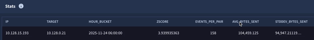
This time, we get a single IP pair and the hourly bucket that appears to be anomalous. We can then start digging into that time bucket to understand what makes this hour different from others for this IP address pair.
The multi-stage search that we just built used a combination of the techniques we introduced in the previous two blogs to build tabled and windowed stages that can be used together to arrive at a more advanced statistical measure. This example can be used as a basis for your own Z-score calculations as it can be broadened to fit other data sets, event types and time windows.
As you build this multi-stage search, keep in mind a few things:
- Each stage except for the root must have a name and is enclosed in curly brackets
- These named stages by themselves do not render an output, so building and testing iteratively is a good approach by adding a root stage to the previous named stage to validate output and then move to the next stage.
- Linkages need to be made between stages. The syntax checker will remind you of this as well, but don’t forget to use $<stage_name> as the variable in front of the field you are using in other stages.
- Only the values in the root stage will be displayed so if you calculated a value in an earlier stage that you want to display, you need to reference it in the root to display it.
This is a more advanced search than the previous ones we looked at but it hopefully illustrates the data analysis techniques that Google SecOps can provide to you. Give it a try with your own network connections or other data sources and see what you might find!