


Last time, I demonstrated how you could build a search in Google Security Operations (SecOps) to create a Z-score to identify outlier IP address pairs and their associated time bucket.
I also mentioned that Z-scores are most meaningful when you have data that falls into a standard distribution, that is the data follows a bell curve. In reality, this is rarely the case. Today, we are going to examine another method to identify outlier behavior, but this time we aren’t going to assume a normal distribution and instead of calculating a standard deviation and a Z-Score, we are going to take a look at using Median Absolute Deviation (MAD).
Median Absolute Deviation
Let’s take a moment to discuss MAD, how it differs from standard deviation as well as why it may be a better choice than its cousin, Mean Absolute Deviation. Standard deviations, which we’ve already used to calculate Z-scores, measure the distance from the mean and then squares the distance before adding the distances up, dividing by the population and finally taking the square root of the result. This result is sensitive to outliers and the effect is compounded by the squaring of the distance. With an outlier or two in the data set, all of the goodness standard deviations can provide may result in a metric that isn’t as useful as it could be if the data was in a standard distribution. And because a Z-score uses the average and the standard deviation, you can see where this could become a problem.
Mean Absolute Deviation addresses this squaring problem by calculating the absolute value from the mean to the data points, sums these deviations and divides that result by the number of data points. Here is how we calculate it:
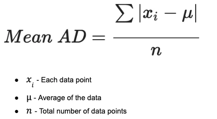
This is a fine approach, but again because we are leaning hard into using the mean in the calculation, an outlier can drastically alter the mean and therefore the results.
This brings us to MAD, which is very similar to mean absolute deviation. The big difference is that the median is used instead of average throughout the calculation, so we are not beholden to an outlier moving the average away from our data set.
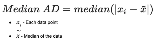
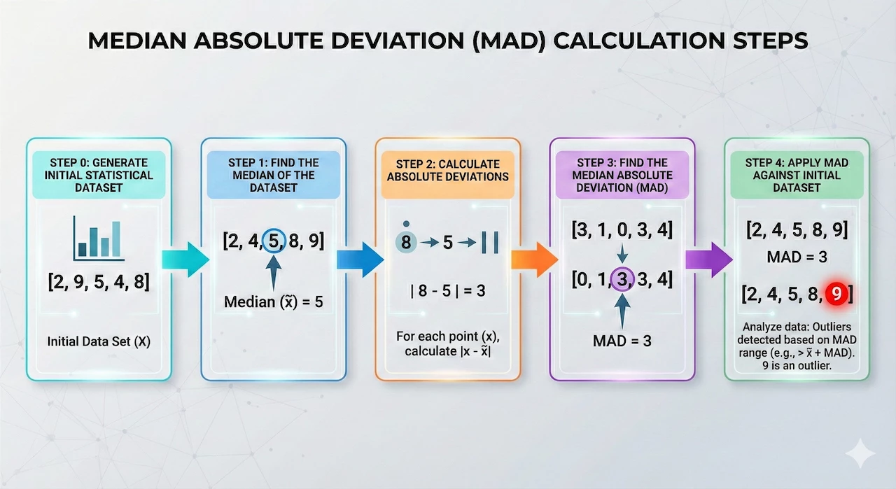
When calculating MAD, we calculate the median of the data set and then calculate the absolute value of the difference between the median and each data point. We then take those differences and calculate the median of the absolute deviations to arrive at the MAD. When we start building our example, we will go deeper into how we approach this, but hopefully this provides a good foundation.
Building a Median Absolute Deviation Search
Much like when we built the Z-score previously, we are going to incrementally build out this multi-stage search, so that we can see the components coming together. It also allows us to iterate and correct any issues we may encounter as we build our logic.
This is a simplified example of calculating MAD, but it provides a useful reference that we can refer back to as we break down the search.
Step 0: Generate the Initial Statistical Data Set
Our first step will be to develop a starter search. This example will evolve into a hunting search for outliers that are communicating within our network for the week of December 20. However, I want to be careful and not throw a bunch of concepts at you with a couple of large netblocks, so let’s start with just a single IP address pair and then once we are happy with our search, we can expand it to a broader data set.
Pro Tip: Whether you are calculating Z-scores, MAD or some other statistical calculation, I generally recommend starting with a smaller data set so that you can validate the content of the search logic to ensure you are arriving at what you expect and then scale it up from there!
We ensure that all of the network connection events have values for sent bytes and we are creating time buckets for each IP pair by hour so we can compare these buckets with one another.
metadata.event_type = "NETWORK_CONNECTION"
net.ip_in_range_cidr(target.ip, "10.128.0.21/32")
net.ip_in_range_cidr(principal.ip, "10.128.15.193/32")
network.sent_bytes > 0
$ip = principal.ip
$target = target.ip
match:
  $ip, $target by hour
outcome:
  $total_bytes_sent = sum(cast.as_int(network.sent_bytes))
  $count = count(network.sent_bytes)
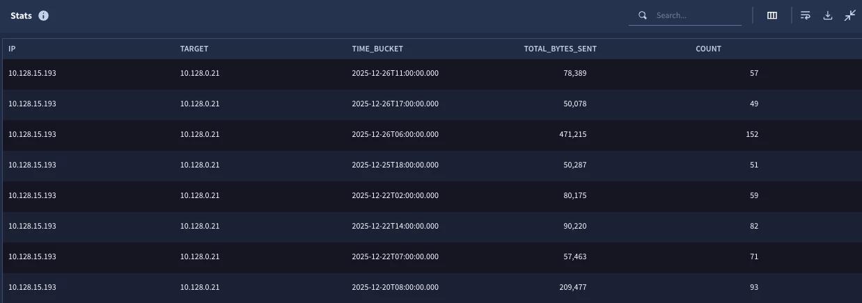
The initial results are a statistical search output with a sum of the bytes sent and a count of the number of events per hourly time bucket per IP. So far, so good.
Step 1: Calculate the Median of the Data Set
We are back to creating a “stat of a stat.” Step 0 created the statistical search to get the hourly buckets and now we need to calculate the median for the IP address pairs across all of the hourly buckets. In our case, we are using a single IP pair, so we will only have a single row in the results.
stage hourly_stats {
metadata.event_type = "NETWORK_CONNECTION"
net.ip_in_range_cidr(target.ip, "10.128.0.21/32")
net.ip_in_range_cidr(principal.ip, "10.128.15.193/32")
network.sent_bytes > 0
$ip = principal.ip
$target = target.ip
match:
  $ip, $target by hour
outcome:
  $total_bytes_sent = sum(cast.as_int(network.sent_bytes))
  $count = count(network.sent_bytes)
}
//root stage
$ip = $hourly_stats.ip
$target = $hourly_stats.target
match:
  $ip, $target
outcome:
  $median_bytes_sent = window.median($hourly_stats.total_bytes_sent, false)
Notice we are simply adding a root stage that is using the IP pair from the first stage, named hourly_stats, and calculating the median in the outcome section. Because we are aggregating by the IP address pair, we get a single row.

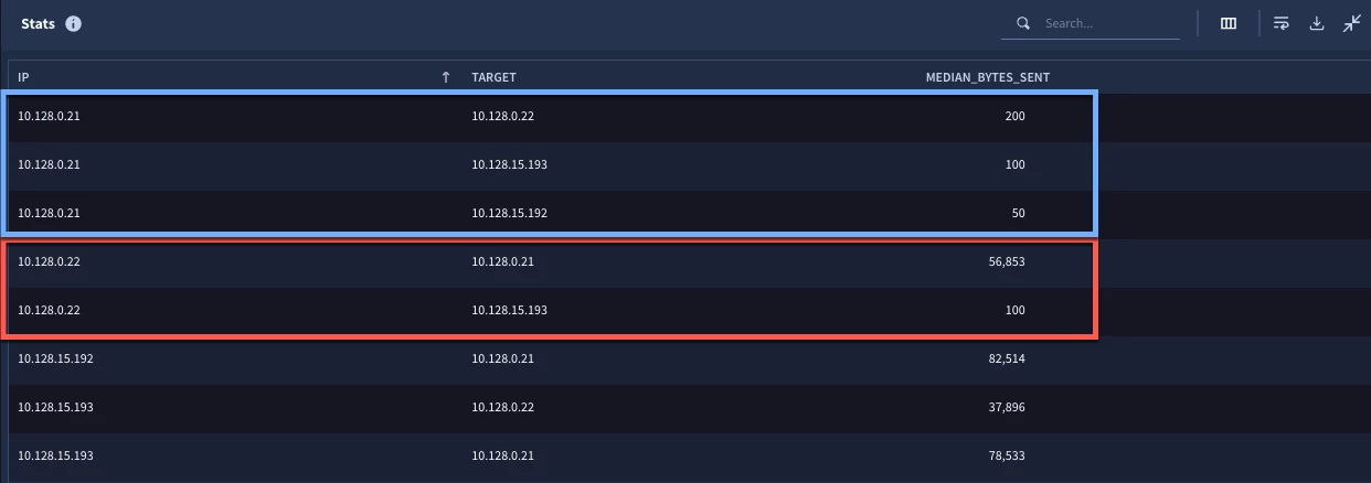
Just in case you are thinking, “Great, but what if we want to calculate the median for more than a single IP pair?”, here are the search results for the same search but with the initial search not limited to a single IP pair. Notice we have a different median value for each IP address pair.
Step 2: Calculating Absolute Deviations
To calculate the absolute deviations, we need two values. The first value is the sum of the network bytes sent for each IP and time bucket. This is in the initial statistical search now in the stage named hourly_stats.
The second value is the median for the IP address pair for the entire time window. We calculated this in Step 1 within the root stage. However, remember that the root stage is the output and really what we want in the output of this step is a series of absolute deviations by hour and IP pair. So, let’s take that median calculation and make it its own stage that we will call agg_stats.
stage hourly_stats {
metadata.event_type = "NETWORK_CONNECTION"
net.ip_in_range_cidr(target.ip, "10.128.0.21/32")
net.ip_in_range_cidr(principal.ip, "10.128.15.193/32")
network.sent_bytes > 0
$ip = principal.ip
$target = target.ip
match:
  $ip, $target by hour
outcome:
  $total_bytes_sent = sum(cast.as_int(network.sent_bytes))
  $count = count(network.sent_bytes)
}
stage agg_stats {
$ip = $hourly_stats.ip
$target = $hourly_stats.target
match:
  $ip, $target
outcome:
  $median_bytes_sent = window.median($hourly_stats.total_bytes_sent, false)
}
// root stage
$hourly_stats.ip = $agg_stats.ip
$hourly_stats.target = $agg_stats.target
$ip = $hourly_stats.ip
$target = $hourly_stats.target
$bucket = timestamp.get_timestamp($hourly_stats.window_start)
match:
  $ip, $target, $bucket
outcome:
  $abs_deviation = max(math.abs($hourly_stats.total_bytes_sent - $agg_stats.median_bytes_sent))
  $total_bytes_sent = max($hourly_stats.total_bytes_sent)
  $median = max($agg_stats.median_bytes_sent)
The agg_stats stage hasn’t changed at all, it’s just named and has curly brackets around it. The new logic in the search is in the root stage where we are joining the IP addresses from the hourly_stats and agg_stats stages together. Joining the IPs is only part of this step however. Keep in mind that in our initial search, we bucketed the total bytes sent by hour. In this stage, we want the output to include each IP address pair, but if we don’t aggregate by time bucket as well, we will end up with a single row. Because of this, we need to add the system created value window_start from the hourly_stats stage. This value became available when we used the by keyword in the match section and grouped by buckets. We can then use this in the match section as part of the aggregation. To make it easy to read, I added the timestamp.get_timestamp function to the field.
Once we’ve done this, the output from the search will be based on each unique combination of IP address pair and time bucket. The calculation of the absolute deviation is very straightforward, just calculate the difference of the total bytes sent in the initial search and the median that was calculated in the agg_stats stage and return the absolute value. Because I like to show my work and make sure that this all lines up as I develop my search, I went ahead and added those two values from the previous stages.
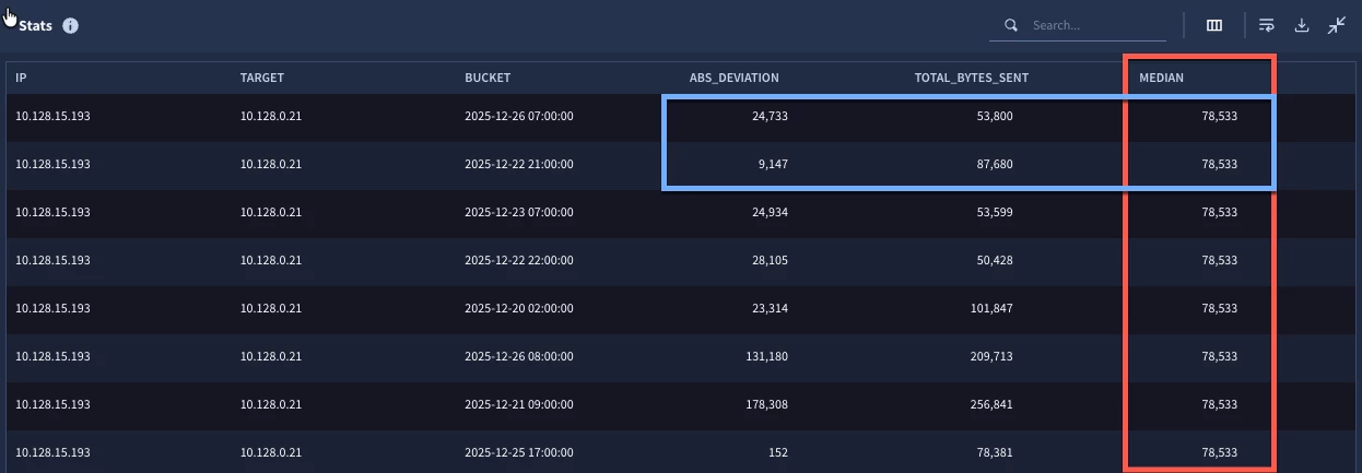
Notice in the results that the median is the same for every row in this result set. With only one pair of IP addresses, that makes sense. If we take the absolute value of the difference of total bytes and the median, we will get the absolute deviation for each row.
Step 3: Calculating the Median Absolute Deviation
With our listing of absolute deviations, we are now in a position to calculate the median absolute deviation for our IP address pair. This is going to be handled much like the way we handled the calculation of the median in step one.
stage hourly_stats {
metadata.event_type = "NETWORK_CONNECTION"
net.ip_in_range_cidr(target.ip, "10.128.0.21/32")
net.ip_in_range_cidr(principal.ip, "10.128.15.193/32")
network.sent_bytes > 0
$ip = principal.ip
$target = target.ip
match:
  $ip, $target by hour
outcome:
  $total_bytes_sent = sum(cast.as_int(network.sent_bytes))
  $count = count(network.sent_bytes)
}
stage agg_stats {
$ip = $hourly_stats.ip
$target = $hourly_stats.target
match:
  $ip, $target
outcome:
  $median_bytes_sent = window.median($hourly_stats.total_bytes_sent, false)
}
stage deviations {
$hourly_stats.ip = $agg_stats.ip
$hourly_stats.target = $agg_stats.target
$ip = $hourly_stats.ip
$target = $hourly_stats.target
$bucket = timestamp.get_timestamp($hourly_stats.window_start)
match:
  $ip, $target, $bucket
outcome:
  $abs_deviation = max(math.abs($hourly_stats.total_bytes_sent - $agg_stats.median_bytes_sent))
  $total_bytes_sent = max($hourly_stats.total_bytes_sent)
  $median = max($agg_stats.median_bytes_sent)
}
//root stage
$ip = $deviations.ip
$target = $deviations.target
match:
  $ip, $target
outcome:
  $mad = window.median($deviations.abs_deviation, false)
As the search continues to evolve, we are taking the prior root stage and making it into a stage called deviations by adding the stage name and curly brackets. In the new root stage, we are defining the IP address pair to use in the match section as the aggregation and then we are calculating the MAD by using the median function. The result is a single value for each IP address pair in the search.

And just like that, we’ve arrived at a MAD calculation for the IP address pair. Now, just because we have a MAD doesn’t mean we are done, we actually need to apply it to our data set to identify the outliers. Otherwise, we’ve basically done the equivalent of creating a standard deviation. We have a value, but what does it mean in the bigger picture?
To find out, I am going to make you wait just a little bit and in the next blog, we are going to come back and take the work we’ve put into this multi-stage search and look at a few different ways it could be applied in your hunts and investigations! In the meantime, give it a try yourself, I’d love to hear how you are using this!

